Deepseek v4.1 flash

# G2C Brief — DeepSeek V4.1-Flash: a model designed around its KV cache

Release question: If an agent spends most of its life reading rather than writing, what should a language model be optimized for?

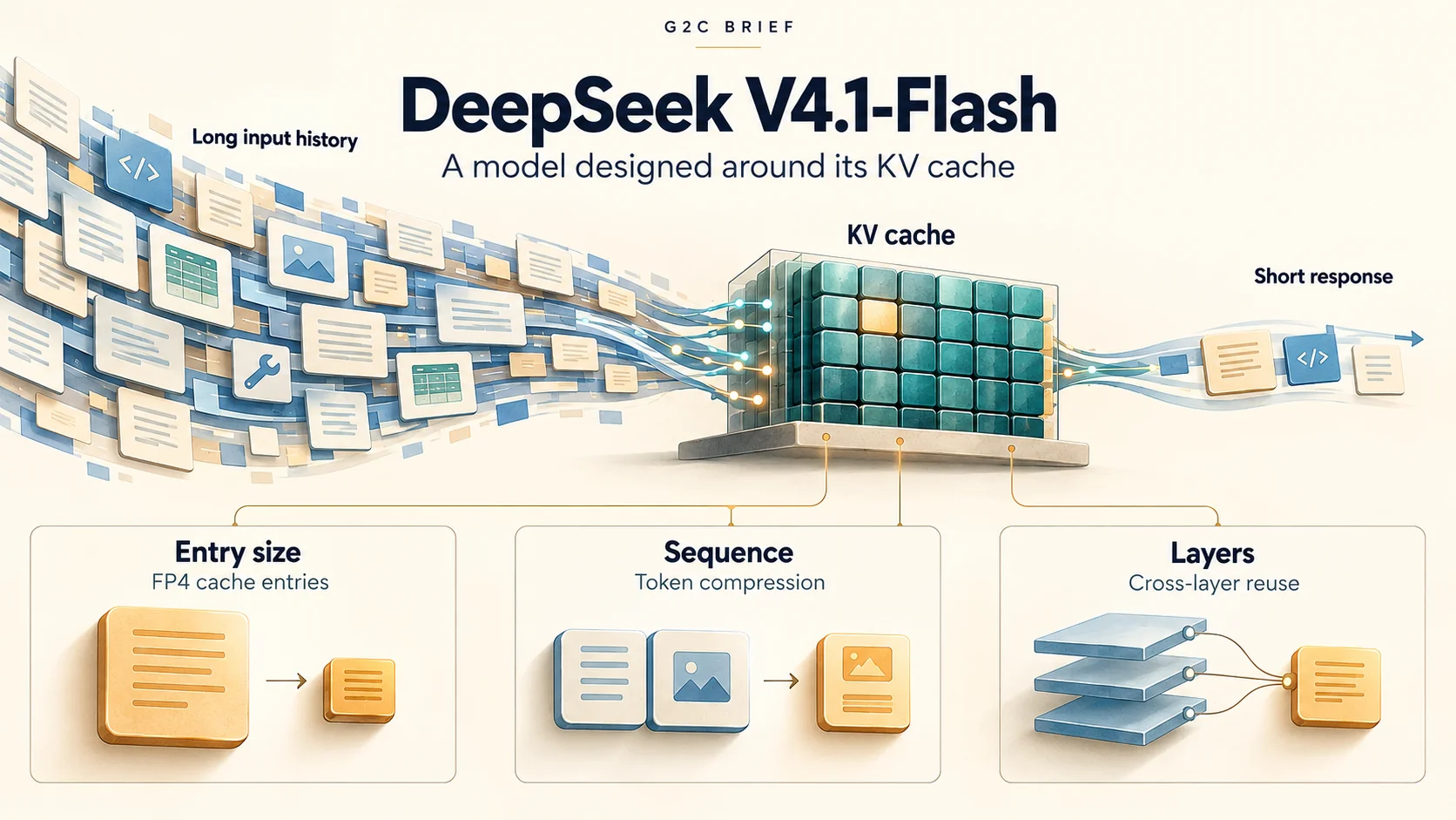
On October 17, 2026, DeepSeek released DeepSeek-V4.1-Flash-1017. It is a new checkpoint of a model family that first shipped five weeks earlier. The update is a modest headline. The architecture underneath it is the more interesting story, and it is unusually readable for someone who has finished g2c.

In Module 16 you wrote forward_cached and a one-line formula for the size of the KV cache. That formula is the design brief for this whole model. DeepSeek's report states plainly that sparse attention has already made long-context compute affordable. The cost that remains is state: the cache for every token an agent has read, which must sit in accelerator memory, spill to SSD, and move across networks. V4.1-Flash is an attempt to shrink that state at every level of the stack: architecture, numerical format, and serving policy.

This Brief assumes you have not read anything about DeepSeek V4 or V4.1. It builds the architecture from pieces you already know, then reads the training, evaluation, and today's checkpoint against that picture.

---

Snapshot

Model family	DeepSeek-V4.1. Flash is the only size released so far; the September release note refers to a forthcoming V4.1-Pro
Checkpoints	DeepSeek-V4.1-Flash, September 10, 2026; DeepSeek-V4.1-Flash-1017, October 17, 2026
Technical report	DeepSeek-V4.1-Flash: Pushing the Limits of KV Cache Compression, arXiv v1 (also in the model repository)
Release notes	September 10 launch · October 17 update
License	MIT, code and weights
Last verified	October 17, 2026

The report describes the September checkpoint. The 1017 checkpoint comes with a model card and a release note but no new report. Everything about architecture and training below comes from the report. The final section covers what is actually new today.

This Brief tags its important claims with four labels, defined in the Brief index. Reported means DeepSeek says so. Derived means arithmetic from disclosed numbers, with the working shown. G2C interpretation means the course's own reading. Not disclosed means the sources don't say. Benchmark scores are all Reported. None of them has been independently reproduced here.

---

The workload that shaped the model

Picture a coding agent twenty turns into a session. Each turn it reads a file, a test log, or a diff. The tool returns a few thousand tokens, the model writes a short reply, and the loop repeats. You built this loop in Module 19. Its token budget is lopsided. Almost everything is input, the conversation prefix is reused on every turn, and the prefix keeps growing.

That workload has three costs, and only one of them is the decode step your sampler runs:

1. Prefill. Every new tool result must pass through the network before the model can respond. If the cached prefix has been evicted, the entire prefix must be prefilled again.
2. Resident cache. While a request is live, its KV cache occupies accelerator memory (HBM). Cache bytes per token × context length × concurrent requests sets how many users a GPU can serve.
3. Persistent cache. To make "the prefix is reused" true across turns and sessions, the server stores caches on SSD or in host memory and reloads them. That costs storage and bandwidth.

Reported. DeepSeek frames V4.1-Flash entirely around these costs: "the primary bottleneck to further lowering deployment costs" is compute, storage, and bandwidth for input-heavy workloads, not raw decode FLOPs.

Your KV formula, pushed to the limit

Module 16 gives the cache size for a vanilla multi-head Transformer:

KV bytes per token = 2 (K and V) × n_layers × n_kv_heads × head_dim × bytes_per_value

The report observes that every way to shrink this multiplies along one of three axes. Each axis is a different kind of trick:

Axis	What you shrink	Familiar example	V4.1-Flash's move
Entry size	bytes stored per cached position	grouped-query attention (fewer KV heads), lower precision	one shared 512-dim latent per position, stored in FP4
Sequence	number of cached positions	sliding windows, token merging	compress groups of tokens into one entry
Layers	how many layers own a cache at all	cross-layer KV sharing	most layers reuse another layer's cache

Derived. The vanilla baseline is easy to compute. A 40-layer model with grouped-query attention (8 KV heads of dimension 128, BF16) stores 2 × 40 × 8 × 128 × 2 = 163,840 bytes, or about 160 KB per token. V4.1-Flash reports 890 bytes per token of global cache, about 184× smaller. The rest of the architecture section explains where that factor comes from.

---

The architecture, piece by piece

The skeleton: a 40-layer MoE Transformer

Start with what is ordinary. Reported. V4.1-Flash is a decoder-only, autoregressive Transformer with 40 layers, hidden size 5,120, a 129,280-token vocabulary, and a one-million-token context window. Every layer has an attention sublayer and a feed-forward sublayer. Images enter through a vision encoder and take positions in the same token sequence as text.

The feed-forward sublayers are mixture-of-experts (MoE). Each one holds 384 small "routed" expert MLPs plus one "shared" expert that always runs. A learned router sends each token to 6 of the 384. Every expert is a SwiGLU MLP with intermediate width 2,304, so it is exactly the FFN from Module 09, only narrower and with many copies.

Derived. One expert has 3 × 5,120 × 2,304 ≈ 35.4M parameters. Then:

routed experts, all layers:  384 × 35.4M × 40 ≈ 544B   (of 552B "backbone")
experts used per token:        7 × 35.4M × 40 ≈ 9.9B   (6 routed + 1 shared)

Nearly the whole parameter count is in experts that any given token skips. That is why MoE models print two sizes. Reported. 552B backbone parameters, 16B activated per token during decoding. Attention, embeddings, and routers make up the gap between the 9.9B expert compute and the reported 16B. The "8B activated during prefill" figure is a separate story, covered in the CED section below.

On top of the backbone sit two more parameter blocks: a 196B-parameter Engram memory and a small speculative-decoding drafter called DSpark. Both come later.

Two attention paths in every layer

Every attention sublayer (except the first two) runs two branches over the same query:

• A local branch: exact sliding-window attention (SWA) over the most recent 128 tokens. This is Module 07's causal attention with a band mask, and it handles fine local detail.
• A global branch: attention over the whole million-token history, made affordable by compression and sparse selection.

The first two layers have only the local branch. G2C interpretation. The report describes the V4 lineage in exactly these terms: an SWA backbone that does local processing, "augmented with compressed global context." Read everything that follows as engineering on that global branch. The local branch is left nearly untouched.

The global branch: compress, index, select

The global branch is called Compressed Sparse Attention. It applies three ideas in sequence:

past tokens   t1 t2 │ t3 t4 │ t5 t6 │ ... │ tN-1 tN       (compression ratio m = 2)
                 ↓       ↓       ↓               ↓
main KV        c1      c2      c3     ...     cN/2         one entry per m tokens
                 ↓  indexer scores every entry for this query (cheap, low precision)
top-k          ■       □       ■      ...      ■           keep the best 512
                 ↓
attention      query attends to the 512 selected entries  +  the local 128-token window

1. Compression. Every m consecutive tokens are folded into one cache entry. Reported. V4.1-Flash uses m = 2 in the first half of the network and m = 1 (no compression) in the second.
2. A shared latent per entry. Reported. Each entry is a single 512-dim vector shared by all 64 query heads (num_key_value_heads = 1, head_dim = 512 in the released config). This is the most extreme version of the "fewer KV heads" idea that Module 08 mentions and puts out of scope.
3. A learned indexer. A small side network with its own low-precision queries and keys (32 heads of dimension 128) scores every cached entry. The query then attends to only the top 512. Attention cost per query stops growing with context. The indexer still scans the whole history, but cheaply.

Built in g2c: scaled dot-product attention, causal masking, and the per-token cache. Conceptual bridge: compression, latents, and top-k selection all reuse those operations. g2c does not build a learned indexer, but Beyond: sparse attention and the efficient-attention map cover the design space.

V4 had a second global layer type with much heavier compression and dense attention. Reported. V4.1 drops it and uses this single scheme everywhere, now called CSA2. It also simplifies the scheme: compressed blocks no longer overlap, and the indexer's keys are now a projection of the main cache entries rather than a separately computed cache.

CSA2: most layers don't keep their own cache

This is V4.1's first big change, and it attacks the layer axis.

Reported. Each CSA2 layer is statically assigned one of three modes:

Mode	Main KV	Indexer K	Top-k selection	Own query + local window
Full	computes its own	computes its own	runs its own indexer	yes
Reindex	borrows from the last Full layer	borrows	re-scores with its own indexer query	yes
Reuse	borrows	borrows	borrows the last selection	yes

Every layer keeps its own query and its own sliding window, so every layer still asks its own question of the context. What gets shared is the stored memory (main KV), and in Reuse mode also the decision about where to look.

The released config shows how sparsely the Full layers are placed:

layer   0  1 │ 2  3  4  5  6  7 │ 8 ... 13 │ 14 ... 19 ║ 20 21 22 23 │ 24 25 26 27 │ ... │ 36 37 38 39
mode   SWA   │ F  R  R  R  R  R │ F  R...  │ F  R...   ║ F  R  R  R  │ X  R  R  R  │ ... │ X  R  R  R
             │      encoder: m = 2, three groups of six │ decoder: m = 1, five groups of four
                                                       F = Full   X = Reindex   R = Reuse

Derived. Only 4 of 40 layers (2, 8, 14, 20) write a global cache. Eight layers run an indexer (the four Full layers plus four Reindex layers). The other 28 attend using a cache and a selection someone else made.

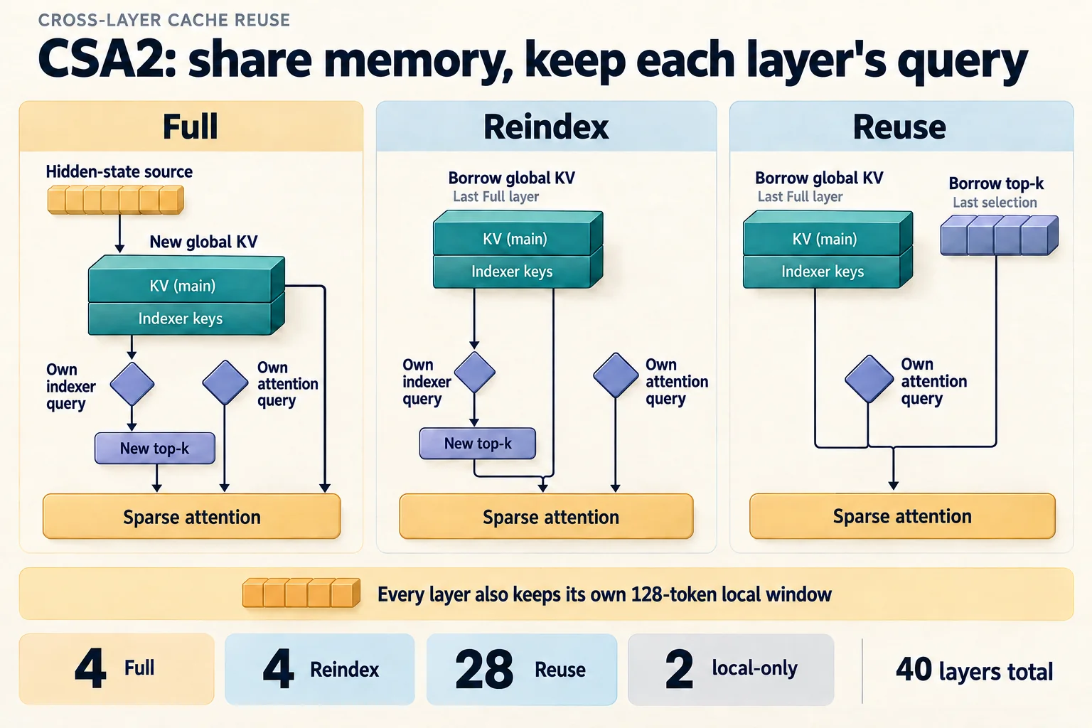Who stores the memory, and who chooses where to look? Reported: CSA2's three modes separate those decisions. Derived: counts follow the released config. The cards compare modes rather than consecutive layers; the hidden-state source follows the CED rule below.

G2C interpretation. This is a strong claim about redundancy. Adjacent layers in a trained Transformer apparently want to look at roughly the same history. They need different queries against it, but not different keys and values. Reported. The report notes that index reuse alone (prior work) saves no storage, and that sharing routing across all layers hurts quality. CSA2 sits between those extremes, with cache sharing and index sharing as separate dials.

The causal encoder-decoder: halving prefill

This is the second big change, and the source of the "8B active during prefill" figure.

First, a naming hazard. "Encoder-decoder" here does not mean the original Transformer or T5. There is no bidirectional encoder and no cross-attention over a separate source sequence. Both halves are causal, and the model is still a single next-token predictor. The report calls the design a Causal Encoder-Decoder (CED), inspired by an earlier architecture called YOCO.

Reported. The 40 layers split into a 20-layer "encoder" and a 20-layer "decoder." In an ordinary Transformer, layer 30's keys and values come from layer 30's hidden state. In CED, decoder layers build their global KV from the encoder's final hidden state H₂₀ instead, through each layer's own projection:

              ┌──────────── ordinary Transformer ────────────┐   ┌────────────── CED ───────────────┐
layer 39      KV₃₉ ← H₃₉                                       │   KV_dec ← H₂₀ · W_KV     (global)
  ...         ...                                              │   SWA KV ← own hidden state (local)
layer 20      KV₂₀ ← H₂₀                                       │   ─────────────────────────────────
layer 19      KV₁₉ ← H₁₉                                       │   encoder layers: ordinary
  ...         ...                                              │
layer  0      KV₀  ← H₀                                        │

The payoff comes during prefill. To build the decoder's global cache for a long prompt, you only need H₂₀ for every prompt token, which means running the bottom 20 layers. The decoder's own hidden states are only needed for tokens the model will actually generate from.

There is one catch. The decoder's local sliding-window branch still uses each decoder layer's own hidden state, and the first decode steps need that local cache. Building it exactly would mean running the decoder over the tail of the prompt. Because a stack of sliding windows widens its reach layer by layer, the tail is the last 128 × 20 tokens. Reported. DeepSeek runs the decoder over only the last 128 prompt tokens and accepts an approximate local cache. They call this Decoder SWA Bounded Replay, and they simulate it during post-training so the model learns to tolerate it.

Derived. For a long prompt, almost every token touches only the encoder. That is half the layers, so roughly half the activated parameters: 16B → 8B. Reported. The report quotes prefill complexity falling from O(N·L) to approximately O(N·L/2).

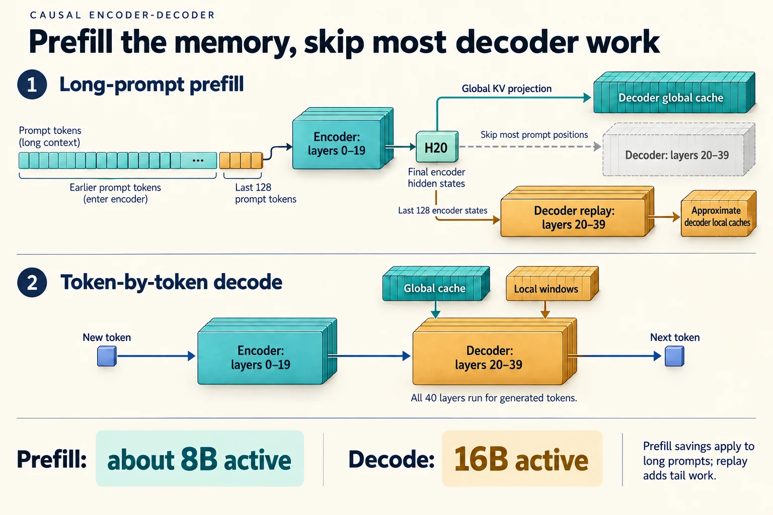The long prompt and generated tokens take different paths. Reported: CED projects decoder global KV from encoder states; bounded replay runs the decoder on the last 128 positions to approximate local state. The 8B prefill figure applies to long prompts; generation and training run all 40 layers.

G2C interpretation. CED is the most direct example in this release of optimizing for the agent workload. In a chat app, prefill is a one-time cost. In an agent loop that appends tool output every turn, prefill is the main event. The final CSA2 picture also follows: decoder layer 20 is the only decoder layer that writes a global cache, and it writes that cache from H₂₀.

The hierarchical indexer: making later indexers context-independent

Even after CSA2 cuts the number of indexers to eight, each still scans the full history. At a million tokens, that scan becomes the bottleneck.

Reported. In the decoder, the first Full layer (layer 20) scores every cached position, as before. It also groups positions into blocks of 8, scores each block by its best member, and keeps the top 2,048 blocks, a pool of 16,384 candidates. Later Reindex layers search only that pool. This feature is introduced in post-training and applied identically in training and inference.

Derived. At a one-million-token context, each Reindex layer scores 16,384 positions instead of about 1,000,000, roughly 1/64 of the work. Unlike the first scan, that cost does not grow as the context gets longer.

Reported. The combined effect, plotted in the report's Figure 2: stretching context 256-fold, from 4K to 1M tokens, raises single-token decode FLOPs by only about a quarter.

FP4 cache entries, and why they're safe

The third attack is on bytes per value.

Reported. Main cache entries are stored as 4-bit floats (E2M1), with one 8-bit (E4M3) scale shared by each group of 16 channels. That is the NVIDIA NVFP4 layout minus its second-level global scale. The model is trained to expect this rounding through quantization-aware training during post-training. The local sliding-window cache stays in FP8 because it proved more sensitive.

The argument for dropping the global scale is worth reading because it is pure Module 09 reasoning. The cache entry is produced after an RMSNorm whose learned weights end up near 1. An RMS-normalized 512-dim vector has L2 norm about √512 ≈ 22.6, so no single channel can exceed that, and RoPE is a rotation, so it preserves the norm. Reported. The observed maximum during training was about 10, comfortably inside FP4-with-scale's range of 2,688. Normalization gives you a numerical guarantee you can design storage around.

Derived: reconstructing the 890 bytes. The released config and the report give every number needed. This Brief assumes the indexer keys use the OCP MXFP4 format the report says V4 adopted (one 8-bit scale per 32 values):

main KV entry:     512 values × 4 bits  + 512/16 scales × 1 B  = 256 + 32 = 288 B
indexer K entry:   128 values × 4 bits  + 128/32 scales × 1 B  =  64 +  4 =  68 B
                                                                 per entry  356 B

encoder: 3 Full layers, m = 2  →  3 × 356 / 2  = 534 B per token
decoder: 1 Full layer,  m = 1  →  1 × 356      = 356 B per token
                                                 ─────
                                                 890 B per token  ✓ matches the reported figure

At the full one-million-token context, that is about 0.93 GB of global cache per sequence. The local sliding-window caches add a fixed amount that doesn't grow with context: 40 layers × 128 positions.

Bounded replay: what to throw away between turns

The last cache trick is a serving policy rather than a model change.

Reported. In V4's deployment, the per-layer sliding-window caches made up nearly half of the persistent (SSD) cache, even though they are only useful for minutes, inside an active session. V4.1 stops persisting them at all. They live in a small, short-lived host-memory pool. If a request returns after they are evicted, the server rebuilds them approximately by replaying only the last 128 tokens of the cached prefix (Encoder SWA Bounded Replay), not the 128 × L tokens an exact rebuild would need.

Reported. Dropping local caches roughly halves the persistent footprint. The 4× smaller global cache supplies the other factor, which gives the headline ~⅛ of V4-Flash's persistent cache. The report finds the approximation "barely compromises response quality."

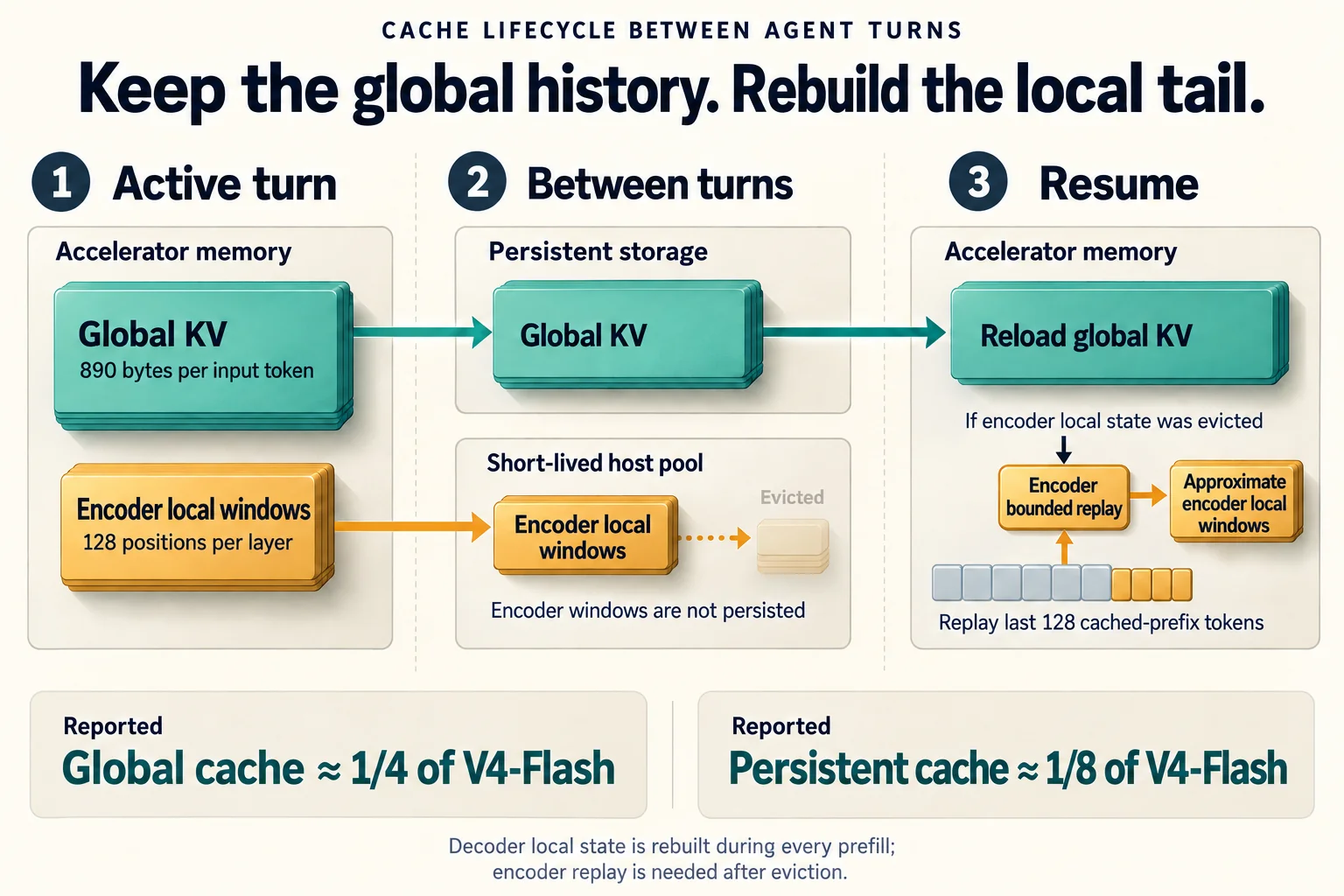What survives between turns determines the storage bill. Reported: the serving policy keeps encoder windows briefly in host memory and rebuilds decoder windows at each prefill. The 890 bytes covers global cache only; the ¼ global and ⅛ persistent comparisons measure different cache categories, both relative to V4-Flash.

G2C interpretation. This is the first place in the stack where the model gives up exactness. After a cache miss, the model's state is no longer exactly what it would have been had the cache survived. The report says so plainly in its limitations section and names "SWA state reconstruction at cache-resumption boundaries" as something it is still stress-testing. Most of what you built in g2c treats the KV cache as an exact memo of a deterministic computation, so this is a real departure.

Four components outside the attention story

These components matter but are not why V4.1 exists. Each gets a short summary.

Engram: a giant hashed n-gram memory. Reported. Two modules, at layers 1 and 14, hold 196B parameters of embedding tables. For each position, the model hashes the preceding 2-, 3-, and 4-token n-grams (8 hash heads per order, tables of about 16M rows) and looks up vectors that are gated into the residual stream. G2C interpretation. This is Module 05's embedding lookup, keyed by short token phrases instead of single tokens. It is memorization stored somewhere other than the experts. Because the addresses depend only on the input tokens, they are known before the forward pass even starts. Reported. That lets the server prefetch the tables from host memory while the first layer computes. The tables never need to live in accelerator memory during serving.

Single-pass mHC: a wider residual stream, fused. Reported. Instead of one residual vector, the model carries four parallel residual streams per token and learns how to mix them around each block. This is called manifold-constrained hyper-connections, and it was introduced in V4. V4.1's change is purely about memory traffic: each block now uses mixing coefficients computed by the previous block. That breaks a data dependency and lets three kernels fuse into one, halving activation reads and writes, at "negligible" quality cost. Module 09 explains why residuals matter. Beyond: mHC covers the multi-stream version.

DSpark: speculative decoding, trained afterwards. Reported. A three-block drafter proposes five tokens at once, and the main model verifies them in one pass. A confidence head predicts how many are likely to survive, and a scheduler sets the verification length to maximize throughput under current server load. V3 and V4 trained their multi-token-prediction module jointly during pretraining. V4.1 drops it from pretraining, trains DSpark separately against a frozen backbone, and keeps updating it during post-training so it also speeds up RL rollouts. The decoding loop you wrote in Module 11 is the thing being accelerated. Standard speculative verification leaves the target model's output distribution unchanged. Not disclosed: the V4.1 report doesn't spell out DSpark's acceptance rule. See Beyond: speculative decoding.

Native vision. Reported. A 32-layer ViT, trained from scratch (first with a SigLIP-style contrastive loss on ~47B image-text pairs, then generatively behind a small 4B MoE LLM). It turns images into patch features. A 3×3 "pixel unshuffle" folds each 3×3 neighborhood into one vector, cutting the token count ninefold, and an MLP projects the result into the language model's hidden size. Images are capped at 1,024 tokens. Image and text tokens get separate router load-balancing biases, because they prefer different experts. See Beyond: multimodal models.

Optimizers, briefly

Reported. Most weight matrices are trained with Muon, which orthogonalizes each momentum update before applying it. Query and key matrices use a per-head variant. The huge embedding-like tables (Engram, token embeddings, output head) use a new Sinkhorn-balanced momentum update that alternately normalizes rows and columns. It needs only one momentum buffer, which matters for 196B parameters of tables. AdamW is kept for norms and biases. Module 03B builds the optimizer contract these plug into. Beyond: Muon covers the orthogonalized update.

---

Training: 45 trillion tokens, then data-driven post-training

Pretraining

Reported.

• 45T tokens, text-only and multimodal at a 7:1 ratio, with images present from the start of language-model pretraining.
• Batch size fixed at 100.6M tokens. Learning rate held at 2.6×10⁻⁴ until 28T tokens, cosine-decayed to 2.6×10⁻⁵ by 40T, then held flat to 45T.
• Sequence length 64K from the start, with sparse attention from step one and no dense-attention warm-up. Extended to 1M tokens at the 34T mark.
• The data pipeline filters out low-value model-generated text, treating it as "implicit duplication."

Derived. 45T / 100.6M ≈ 447,000 optimizer steps. A rough Module 12-style compute estimate, 6 × N_active × D with N = 16B and D = 45T, gives about 4×10²⁴ FLOPs. That ignores attention, Engram, vision, and the 1M-token stage, so read it as an order of magnitude only. Training runs every token through all 40 layers (the loss needs the decoder), so the 8B prefill figure doesn't apply here.

Reported. The base model matches V4-Pro-Base, a 1.6T-parameter, 49B-active predecessor, on most knowledge and reasoning benchmarks. A few selected rows:

Base model	V4-Flash	V4-Pro	V4.1-Flash
Activated / backbone params	13B / 284B	49B / 1.6T	8–16B / 552B
MMLU-Pro	68.3	73.5	74.1
SimpleQA-Verified	30.1	55.2	42.3
HumanEval	69.5	76.8	79.4
MATH	57.4	64.5	61.1
LongBench-V2	44.7	51.5	45.2

G2C interpretation. Look at where V4.1-Flash falls short of V4-Pro: SimpleQA (factual recall) and long-context reading. Parameter count still buys memorized facts, as Module 15 would predict.

Post-training: "no algorithmic innovation"

This is the most quotable sentence in the report, and a good lesson to take away from the course. Reported. The post-training recipe is SFT, then RL, then on-policy distillation, "without any modification beyond well-established practice." DeepSeek attributes "essentially all" of the gains to the data: synthesized tasks, environments, and verifiers.

What that data pipeline looks like (Reported):

• Tasks as triples. Every RL task is a (problem, environment, verification system). The model is itself trained, with RL, to construct tasks, rewarded for difficulty and correctness. This is Module 16B's synthetic-data loop, closed and running at scale.
• Agent-built coding environments. Separate agents decide whether a GitHub repo can be containerized and auto-verified, write fail-to-pass tests, set up the container, attempt the task, inspect the environment for hackability, and repair it. Tasks that fail inspection are recycled.
• Mocked tools from real usage. Employee and partner workflows are turned into mock SaaS and back-end tools. Reported failures become new RL environments.
• Millions of concurrent sandboxes. During RL, agents tried to escape or game their containers. The report lists exploiting filesystem-driver bugs, pulling answers from package mirrors, and deleting system files. Crashes are scored as failures. Module 18's sandboxing advice, at production scale.
• Model merging between RL runs. Checkpoints from runs on different agent scaffolds are merged, and the merge seeds the next run.
• On-policy distillation from 40+ teachers. The final stage distills from more than 40 domain-specialist teacher models into the single student, using the full output distribution.

A reasoning-effort dial trained into the weights. This is the one post-training mechanism you can write down completely. Reported. The system prompt carries Reasoning Effort: {b} with b from 1 to 100. During RL, responses are grouped by (prompt, effort level) and advantages are computed within each group, GRPO-style. The reward includes a length penalty whose strength decays exponentially with b:

r_len = −min( C_max,  k(b) · ℓ / L_norm ),        k(b) = k₀ · exp( −(b − b_min) / τ )

Low effort means expensive tokens, so the model learns to stop early. High effort means cheap tokens, so it explores. The API's low / high / max tiers are b = 50 / 75 / 100. Reported. Going from effort 25 to 100 raises average accuracy on eight reasoning benchmarks from 67.1% to 76.3%, at about 2.5× the output tokens. Effort 60–80 recovers most of the gain at under half the tokens of max. Conceptual bridge: Module 14 covers preference optimization and Beyond: RLVR with GRPO covers group-relative advantages. The effort dial is a reward-shaping layer on top of both.

---

Reading the evaluations

Reported. Selected instruct results at maximum effort, as published in the report. Comparison scores are DeepSeek's own runs or citations.

Benchmark	V4-Flash	V4-Pro	V4.1-Flash	Best listed closed model
GPQA Diamond	89.9	92.4	90.9	94.1 (GPT-5.6 Sol)
Terminal-Bench 2.1	82.7	87.9	90.6	89.1 (Opus 5)
Terminal-Bench 4.0	7.0	12.4	31.2	51.8 (Opus 5)
DeepSWE v1.1	54.4	62.7	74.2	74.0 (Opus 5)
Automation-Bench	37.7	43.2	54.8	50.3 (Opus 5)

Three things to read in this table, using Module 15's habits:

1. The jump is in agentic coding, not knowledge. GPQA barely moves from V4-Flash. DeepSWE gains 20 points. That fits a release whose improvements are attributed to RL environments, not pretraining scale.
2. The report names its own weak spot. DeepSeek acknowledges a remaining gap on science-heavy agent tasks such as Terminal-Bench 4.0. The 20-point shortfall against the best closed model there is consistent with the base-model gap in factual recall above.
3. The harness is part of the score. Reported. The same checkpoint on DeepSWE v1.1 scores 74.2 in the mini-SWE harness, 72.6 in DeepSeek's own harness, 69.8 in Claude Code, and 65.5–66.2 in OpenCode, Pi, and Codex. A 9-point spread from the wrapper alone is a concrete version of the Module 19 and Module 20 lesson: agent benchmarks measure model + loop, never the model by itself.

---

What's new today: the 1017 checkpoint

Derived. The config.json in the 1017 repository is byte-identical to the September checkpoint's, and the safetensors parameter counts match by dtype. This is the same architecture with new weights. Everything above applies unchanged.

Reported. The model card calls it "a minor update" with gains across reasoning, coding, agentic, and visual tasks, plus shorter outputs and faster task completion. The release note attributes the project-building gains to "reinforcement learning with self-feedback." Selected rows:

Benchmark (model card)	V4.1-Flash	V4.1-Flash-1017	Change
HLE (no tools)	36.8	42.6	+5.8
Terminal-Bench 4.0	31.2	42.3	+11.1
DeepSWE v1.1	74.2	77.0	+2.8
ProgramBench	20.3	29.1	+8.8
Automation-Bench v1.0.6	54.8	60.5	+5.7
Apex Bench v1.1	64.6	72.1	+7.5
BabyVision (with tools)	89.6	92.5	+2.9

(The "Change" column is Derived. The card also lists GLM-5.3, K3, GPT-5.6 Sol, and Opus 5. Among its 11 rows, 1017 leads on DeepSWE, Automation-Bench, Agents' Last Exam, and Apex Bench. Opus 5 or GPT-5.6 Sol leads on the other seven, including HLE, Terminal-Bench 4.0, and ProgramBench by wide margins.)

G2C interpretation. The largest gains land on the long-horizon benchmarks (Terminal-Bench 4.0, ProgramBench), which is where the report admitted the September model was weakest. Better scores combined with shorter outputs suggest more RL of the same kind, with length pressure from a penalty like the effort dial's. The sources don't say how it was trained, so treat that as a hypothesis.

Not disclosed:

• What "RL with self-feedback" means: who produces the feedback, how it becomes a reward, and whether the data pipeline changed.
• Output-length numbers. The release note's charts are images with no figures in the text.
• Whether the September column was re-run under the card's stated harness. The card says Terminal-Bench 4.0 used the Claude Code harness, while the report says code-agent benchmarks used DeepSeek's own harness. Both show 31.2 for September, so it is unclear whether that baseline was re-measured.
• Any change to safety behavior or long-context robustness. The card makes no claim about either.

One serving detail changed: the 1017 card recommends top_p = 1.0. The September card allowed 0.95 or 1.0, and the report's evaluations used 0.95. After Module 11 you can read that as "sample from the full distribution at temperature 1.0, with no nucleus truncation." The card gives no reason for the change.

The same release opened DeepSeek's in-house Search and Fetch APIs to the public. That is a product change for agent builders, not a model change, and this Brief doesn't cover it.

---

The laptop boundary

You will not run this model on a MacBook, and this Brief does not ask you to. Derived. The released safetensors files hold about 765 GB of tensors (2 × 1.98B BF16 + 4 × 0.04B FP32 + 204B FP8 + 557B 8-bit elements, in bytes). That is more than ten times the largest unified-memory configuration in the course's hardware contract, and serving it assumes multi-GPU expert parallelism.

What is within reach is reading it. The repository's inference/model.py is a self-contained reference implementation under MIT. With your own TransformerLM from Module 10 open beside it, the CSA2 mode dispatch, the CED projection from H₂₀, and the Engram lookup are legible as diffs against code you wrote.

---

Coverage map

Mechanism	Label	Where to anchor it
Decoder-only Transformer, causal attention, RoPE, RMSNorm, SwiGLU	Built in g2c	Modules 07–10
KV cache and its size formula	Built in g2c	Module 16
Sliding-window attention	Conceptual bridge	Module 07's causal mask, banded
Shared-latent KV (one KV head, 512-dim)	Conceptual bridge	Module 08 (GQA noted as out of scope)
Token compression + learned top-k indexer (CSA2)	Conceptual bridge	Beyond: sparse attention
Cross-layer KV and index reuse (Full/Reindex/Reuse)	Not yet covered	Efficient-attention map
Causal encoder-decoder (YOCO-style KV from a middle layer)	Not yet covered	Module 16 (why prefill matters)
Hierarchical sparse indexer	Not yet covered	—
FP4 cache + quantization-aware training	Not yet covered	Beyond: hardware
SWA bounded replay / persistent cache policy	Conceptual bridge	Module 16
Mixture-of-experts routing and load balancing	Conceptual bridge	Beyond: MoE
Engram hashed n-gram memory	Conceptual bridge	Module 05 embeddings
mHC multi-stream residuals	Conceptual bridge	Beyond: mHC
DSpark speculative decoding	Conceptual bridge	Module 11, Beyond: spec. decoding
Vision encoder + projector	Conceptual bridge	Beyond: multimodal
Muon / Sinkhorn-balanced updates	Conceptual bridge	Module 03B, Beyond: Muon
SFT → RL → on-policy distillation	Conceptual bridge	Modules 13, 14, Beyond: RL
Synthetic tasks, environments, verifiers	Conceptual bridge	Module 16B
Agent harnesses and sandboxing	Conceptual bridge	Modules 18–20, Beyond: harness

---

What the report itself flags as open

The report's limitations section is unusually specific, and worth quoting in substance. Reported. It notes that the new architecture "creates robustness boundaries that have yet to be fully characterized." Two risks are named: selection errors in CSA2, where the indexer misses an entry that mattered, and approximate state reconstruction in bounded replay. It also cautions that benchmark parity with frontier closed models "does not imply that the model matches" them on the hardest tasks.

G2C interpretation. Both named risks have the same shape. They are places where the model swaps an exact computation for a cheaper, learned approximation, and they will fail rarely, on inputs that no benchmark happens to sample. "Find the one line in a 900K-token log that matters" tests the indexer. "Resume a session after the cache was evicted mid-task" tests the replay. If you want to probe the model yourself, those are the two places to look.

---

A reading route

If you have an hour with the report, read it in this order:

1. §1 Introduction, for the three-cost framing (prefill, resident cache, persistent cache).
2. §2.2–2.3 (CED, CSA2), with this Brief's layer map open. Figure 4 is the clearest single picture of the three modes.
3. §2.4.4 (FP4 cache), for the norm-bound argument.
4. §3.2 (inference system), for bounded replay and the persistent-cache policy.
5. §5.1.1 and §5.1.4, for task synthesis and the effort dial.
6. §5.3.4, Table 4, for the harness spread, then the 1017 model card.

Skip §3.1 (distributed-training plumbing) and the optimizer derivations unless those are your interest.

After this Brief, you should be able to

• Explain why input-heavy agent workloads make KV-cache state, not decode FLOPs, the binding cost.
• Name the three axes of KV compression and say which V4.1 mechanism works on each.
• Explain how a "causal encoder-decoder" differs from a T5-style encoder-decoder, and why it halves prefill.
• Reproduce the 890-bytes-per-token figure from the config and the cache formats.
• Say which parts of V4.1 trade exactness for cost, and what failure would look like.
• Read the 1017 update as "same architecture, more post-training," and list what its release does not disclose.