Beyond — Mixture of experts

Question this module answers: How can a model store far more parameters than any one token uses?

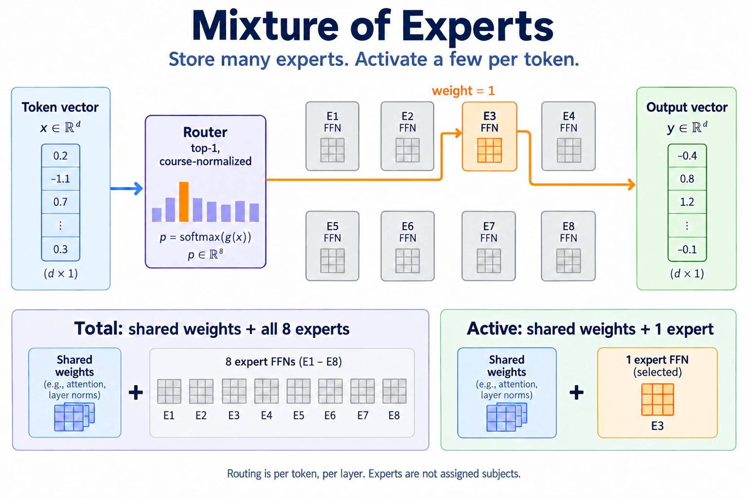
This week introduces a new variant of the classic transformer architecture. Up until now, we have described models with a single parameter count. MoE asks us to track two: total parameters and active parameters. Done well, it gives a model substantially more parameter capacity without making every token use all of it.

This is a Beyond module. Beyond modules sit outside the numbered course: nothing in Modules 00–20 depends on them, and they are not part of finishing the course. Come here in any order, whenever a model card or paper names the idea and you want the load-bearing version — built, trained, and broken on your own machine.

---

Before you start

• Review
  • 09-transformer-block for the FFN and Block anatomy
  • 12-scaling for parameter and FLOP accounting
• Finish
  • g2c/transformer (09-transformer-block)
  • g2c/training (03b-training)
• Run
  • ./datasets.sh --tiny if the TinyStories corpus or StoryTokenizer artifact is missing
  • G2C_APPLY_SOLUTIONS=01-11 ./notebook.sh moe instead of the plain launch if you're entering without your own Part I implementations

---

Where this fits in

Module 09 taught you that the feed forward network (FFN) is the "compute" half of the transformer block. Module 12 taught you where the parameters live: roughly two-thirds of a transformer block's weights are in its FFN. Put those together and a dense transformer has an awkward property — every token uses every FFN weight in every layer. If you enlarge those FFNs to add capacity, every token's forward pass gets proportionally more expensive.

The tension comes down to the scaling laws you explored in Module 12: larger models generally have more capacity, but a dense model applies all of its layer weights to every token. MoE asks whether conditional computation can provide more capacity at roughly the same per-token compute. It is tempting to imagine one expert for Python and another for children's stories, but learned experts are rarely that tidy. Their specializations emerge from training and may reflect token roles, local syntax, or patterns that are difficult to name.

Mixture of experts (MoE) is an architectural variant of the transformer block that applies this idea. It trains a large parameter set while activating only a fraction of those parameters for each token. The expert networks can learn different functions, and tokens are routed according to their current context.

One common misconception is that expert networks are explicitly assigned subject matter data. They are not: experts begin as architecturally interchangeable sub-networks in the block. MoE networks use the same pretraining objective introduced in Module 09B, and specialization may emerge through gradient descent—often in opaque ways.

The big idea

Keep the block, keep the attention, keep the residual stream — but replace the single FFN component with E independent FFNs ("experts"). Put a small learned router in front of each expert layer. For each token, the router selects k experts to activate. Do this in every transformer layer and you have an MoE.

   Dense block (Module 09):            MoE block (this module):

   x ─► LN ─► MHA ─► + ─┐              x ─► LN ─► MHA ─► + ─┐
                        │                                   │
   ┌────────────────────┘              ┌────────────────────┘
   │                                   │
   x ─► LN ─► FFN ─► + ─┐              x ─► LN ─► router ─┬─► FFN₁ ─┐
                        │                        (top-k)  ├─► FFN₂ ─┤
                        ▼                                 ├─► ...  ─┤  
                     (B, T, D)                            └─► FFN_E─┤
                                                                    │
                                                                weighted +
                                                                    ▼
                                                                (B, T, D)

One dense FFN becomes E candidate FFNs plus a router. Per token: the router scores all E experts, keeps the top k, runs those k FFNs, and combines their outputs weighted by the router's (renormalized) scores. Everything else in the block is untouched.

Capacity now scales with E. Per-token compute scales with k. Those are the two numbers on the model card: total parameters count every expert, active parameters count only the ones a token actually touches.

Activation routing runs per token because the FFN operates per position. It never mixes information across tokens. Nothing breaks semantically if token 3 and token 7 go through different experts — there is no attention mask to maintain or KV cache to invalidate. Implementations still gather, batch, and dispatch tokens by expert, and frontier systems may enforce per-expert capacity across a batch. Those are execution concerns rather than cross-token dependencies in the model function. Attention is the communication half that must see everyone; the FFN is the compute half that is free to specialize.

Each transformer layer maintains its own independent expert panel and router, so specialization can differ by layer. Combined with per-token routing, this means specialization happens at a much finer granularity than the full prompt. For example, a 64-layer network processing a 1,000-token prompt makes 64,000 independent routing decisions during the forward pass.

The router

The router is deliberately boring. It takes the residual stream as input and outputs sparse weights across the experts in the block. Those weights determine which expert FFNs are activated and how their outputs are mixed back into the residual stream. During gradient descent, the router learns context-dependent routing scores alongside the experts.

The router has a simple internal architecture: one linear layer followed by three operations that create the activation properties we want:

• Softmax. Softmax turns the raw logits into a categorical distribution over experts.
• Top-k. The operation that keeps activation sparse. Without it, every expert would receive a non-zero weight.
• Renormalize. This module rescales the surviving weights to sum to 1 after discarding all but k. For k>1, this preserves their relative differentiable strength. k=1 is an important edge case covered more in the next section.

   scores  = softmax(x_t @ W_router)        # (E,) — one score per expert
   top-k   = indices of the k largest       # e.g. k = 2
   weights = renormalize(scores[top-k])     # this module's mixing rule

   output  = Σ  weights[e] · FFN_e(x_t)     # over the k selected experts

The selected top-k indices are not differentiable. This creates complications for gradient descent that must be managed carefully. If k > 1, each token has multiple surviving experts with differentiable relative weights, so the language-modeling loss can still send a learning signal to the router through those weights.

Top-1 conventions

Top-1 systems differ in what they do with the winning probability p_e. This one detail determines whether the task loss can train the router:

Convention	Output for selected expert e	Task gradient to router	Main tradeoff
Course-normalized top-1	FFN_e(x)	None through the mixture weight	Stable output scale and exact E=1 dense equivalence
Switch-style top-1	p_e · FFN_e(x)	Yes, through p_e	Output scale depends on router confidence

In both cases, the discrete winning index remains non-differentiable. Switch-style weighting retains a local surrogate signal through the selected probability; it still does not evaluate the unselected experts and directly reveal which counterfactual route would have been best.

This distinction limits what the headline k=1 experiment can demonstrate. Its auxiliary loss can move the router toward a more even input-dependent partition, ensuring that every expert receives training traffic. But it carries no task signal about which expert would have predicted a token best.

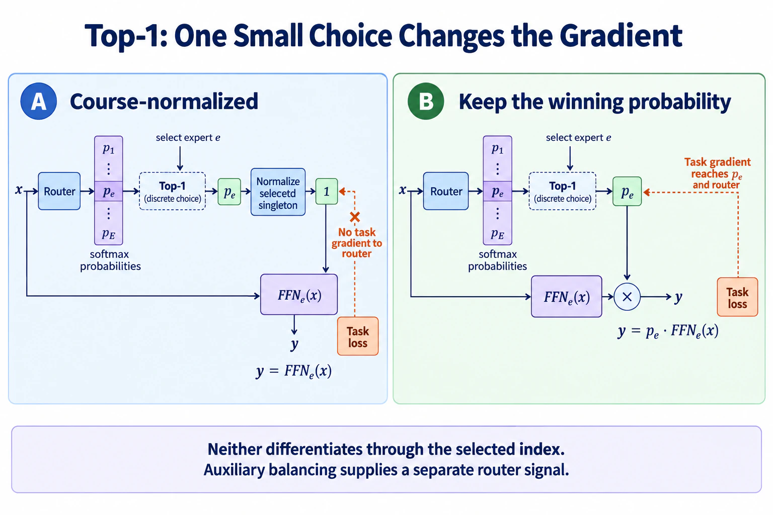The selected index is discrete in both cases. What changes is the surviving mixture weight—and therefore whether the task loss can train the router before the balancing loss is added.

Load balancing

For both k=1 and k>1, router training can be pathological under the standard language-modeling loss. As we saw above, a renormalized k=1 router receives no useful task gradient and remains near its initialization without another objective. For k>1, a task gradient exists, but training can drift toward router collapse.

Router collapse is a classic rich-get-richer scenario. Whichever expert becomes slightly favored during training receives more traffic and gradient, which can make that route still more attractive. Left unchecked, one or two experts may become overworked while the rest receive too little training.

A standard countermeasure is a supplemental term added to the training objective. An auxiliary load-balancing loss penalizes uneven expert use across the token distribution:

   f_e  =  fraction of tokens routed to expert e        (hard counts)
   P_e  =  mean router probability for expert e         (soft scores)

   L_balance  =  E · Σ_e  f_e · P_e

Uniform routing gives the reference value 1 (f_e = P_e = 1/E for all e), while aligned collapse approaches E. The expression is a surrogate rather than a distance metric: 1 is not a strict lower bound for every finite batch because the hard assignment frequencies and mean soft probabilities can be imperfectly aligned. Its useful property is the gradient: overused experts contribute more through f_e, pushing their mean probability P_e down and restoring a router-training signal even for k=1.

The auxiliary loss is weighted by a small coefficient and added to the language-modeling loss. The coefficient represents a genuine tension, not a nuisance parameter. Too low permits concentration. Too high can force routing toward uniformity and crowd out useful specialization. Like any hyperparameter, it should be swept and chosen from empirical evidence.

Counting total vs active

Let's revisit the parameter accounting from Module 12. For embedding dimension D, a transformer block has approximately 12·D² parameters: 4·D² in attention and 8·D² in the FFN.

In an MoE block, the attention component remains the same. But with E experts you now have E FFNs, each with 8·D² parameters. The router adds another D·E + E parameters when its linear layer includes a bias, usually a negligible contribution at model scale.

   dense block:    4·D² (attn)  +  8·D² (FFN)              ≈ 12·D²

   MoE block:      4·D² (attn)  +  E·8·D² (all experts)  + D·E (router)
        total  ≈   4·D²  +  E·8·D²
        active ≈   4·D²  +  k·8·D²      ← what one token's forward pass costs

With this module's default E = 8, k = 1, total block parameters grow ~5.7× while active block parameters remain approximately equal to the dense block. One dense FFN has simply become one selected expert of the same width. The routers add a small amount of active work, so the counts are near-matched rather than bit-identical.

Scale the same arithmetic up and you can begin to decode a model card. V4-Flash's 284B total / 13B active split signals a large gap between stored capacity and per-token activation, though those two numbers alone do not reveal the expert count or width. FLOPs track the active count much more closely than the total count, while the total count conveys parameter capacity and storage requirements. This remains an approximate picture: routing overhead, memory movement, batching, and hardware all affect real latency and API price.

MoE refinements in practice

Several refinements commonly accompany MoE models. They're worth recognizing by shape:

• Shared experts — One or two universal experts that every token goes through, in addition to the specialized routed ones. They handle common computation, giving the routed experts more room to differentiate.
• Fine-grained experts — Use a larger number of smaller experts for a similar parameter budget. Instead of 8 large experts, choose 64 smaller ones and route to more of them on each pass. This provides finer routing granularity. Kimi K3's "16 of 896" routing shape is a frontier-scale example, though its LatentMoE experts add machinery beyond the direct FFN swap built here.
• MoE placement — Not every model replaces every FFN. Some keep the first few layers dense, alternate dense and MoE blocks, or route only selected layers. A model card's expert count therefore does not tell you how many routing decisions occur per token; you also need the number and placement of MoE layers.

All three are straightforward to recognize once the base mechanism is built. This module leaves them out so the scaffold retains the simplest routed-FFN shape.

Concepts to internalize

• MoE decouples capacity from per-token compute. Total parameters are a capacity and storage measure; active parameters are a closer proxy for what each token costs. In dense layers, all layer weights are active for every token.
• The FFN is swappable because it's per-position. No cross-token machinery has to change. This is why MoE lives in the FFN and not (usually) in attention.
• Router learning depends on the mixing convention. With renormalized k>1, relative combination weights carry a task gradient. Course-normalized top-1 removes that signal by setting its sole weight to 1; Switch-style top-1 retains the winning probability and therefore retains a task gradient.
• Balanced routing is not the natural state. With k>1, rich-get-richer collapse is possible; with this implementation's k=1, an unbalanced random partition can simply stay frozen. The auxiliary loss is a counterweight you tune, not a formality.
• Model-card literacy: "X total / Y active" ⇒ per-token compute usually tracks Y much more closely, while storage follows X. Compare MoE and dense models at matched active parameters, not matched total.

What we don't cover

• Expert parallelism and communication. At frontier scale the experts live on different devices and the routing becomes an all-to-all network problem. That's distributed-systems engineering the course explains but doesn't reproduce — our experts share one chip.
• Capacity factors and token dropping. Large-batch training bounds how many tokens each expert may receive and drops the overflow. At our batch sizes it's machinery without payoff.
• Auxiliary-loss-free balancing. DeepSeek-V3 balances with a per-expert bias adjusted outside the gradient instead of an aux loss. A neat variation; read it after building the standard form.
• Router noise and logit stabilization. Some recipes add random jitter or noisy routing to improve exploration, and a router z-loss to discourage excessively large logits. These address exploration and numerical stability; they are distinct from the load-balancing objective implemented here.
• Latent-width and low-rank expert variants (e.g. the LatentMoE line). Refinements of where the expert computation happens, not of the routing idea; they read easily once this module is done.

---

What you'll build

Package: g2c/moe/

class Router(Module):
    embedding_dim: int
    num_experts: int                     # E
    top_k: int                           # k
    gate: Linear                         # (D, E)

    def parameters(self): ...                                   # implemented
    def forward(self, x): ...                                   # SCAFFOLDED
        # returns (weights, indices): (B, T, k) each —
        # softmax over E, top-k selection, renormalized weights

class MoEFeedForward(Module):
    embedding_dim: int
    num_experts: int
    top_k: int
    experts: list[FeedForward]           # E copies of Module 09's FFN
    router: Router

    def parameters(self): ...                                   # implemented
    def forward(self, x): ...                                   # SCAFFOLDED
        # dispatch each token to its k experts, weighted-sum the outputs;
        # record routing fractions for the balance loss
    def load_balancing_loss(self): ...                          # SCAFFOLDED
        # E · Σ_e f_e · P_e from the last forward's routing stats

class MoEBlock(Module):                  # Block with the FFN swapped     # implemented
class MoETransformerLM(Module):          # TransformerLM over MoEBlocks   # implemented

Total scaffolded code: roughly 30 lines across three methods. The dispatch in forward is written as a legible loop over experts — gather the tokens routed to expert e, run them, scatter the results back. Production systems fuse this into batched kernels; we keep the loop because you can read it.

How to run the tests

Tests live in tests/test_moe.py. Initial state: 9 passed (construction, accounting, and validation checks), 13 failed.

source .venv/bin/activate

pytest tests/test_moe.py                 # all MoE tests
pytest tests/test_moe.py -x              # stop at first failure (recommended)
pytest tests/test_moe.py -k router       # router tests only
pytest tests/test_moe.py -k balance      # load-balancing tests only
pytest tests/test_moe.py -v              # verbose

The anchor test to know about: test_moe_e1_k1_matches_dense asserts that an E = 1, k = 1 MoE layer is numerically identical to Module 09's plain FFN. If your dispatch logic is right, MoE with one expert is the dense model — a strong sanity check that costs nothing.

Exercises

To launch the exercise notebook run:

./notebook.sh moe

If at any point you want to archive the work in your current notebook and restart fresh:

./notebook.sh moe --fresh

Written exercises live in the notebook as Question: / Answer: cells; ask a coding agent for hints or grading when you're ready, and partial submissions are fine — blank answers are skipped.

1. Collapse to dense. Verify E=1, k=1 reproduces the Module 09 block, then read the routing weights of an untrained E=8 router.
2. Matched-active comparison. Train dense and MoE versions of the StoryLM-1M architecture on the 100MB TinyStories tier, with E=8, k=1, iso-step, and identical batches. Compare validation loss, parameter counts, and generated stories. This is the module's headline capacity experiment: it isolates conditional computation at near-matched active size, but its course-normalized top-1 router is not task-trained. The router is the only meaningful active-parameter difference.
3. Top-1 utilization over training. Plot the per-expert token fraction in the matched-active run. Because renormalization makes the selected k=1 weight exactly 1, changes in its router come from the auxiliary loss rather than the language-modeling objective.
4. Ablate the balance loss with k=2. Compare three otherwise-identical MoE runs: coefficient 0, the calibrated default, and 100× the default. This is the module's task-trained routing experiment: the language-modeling loss can reach the router through the relative weights of the two selected experts. The first permits task-driven concentration; the last can force routing so uniform that specialization has little room to emerge. Keep all three plots even if a short run produces a weaker effect than expected — the empirical result is the evidence.
5. Sweep k (optional). Compare k ∈ {1, 2, 4} at fixed E. More active experts per token means more compute per token — is it buying loss?
6. StoryLM-5M rerun (optional). Repeat the matched-active comparison with the StoryLM-5M architecture. The model is still laptop-sized, but its eight-expert MoE holds roughly 28M total parameters and the extra runs take substantially longer.
7. Specialization probe (optional). Bucket decoded TinyStories tokens by expert assignment and look for structure. At toy scale the buckets may be noisy; an honest null result is more useful than inventing a role for every expert.

Pitfalls to expect

• Forgetting the course's renormalization rule. With k>1, output scale then depends on how much probability mass survived selection. The dedicated router weight-sum test catches this; E=1, k=1 cannot, because a one-class softmax already equals 1. Retaining the winning probability in a deliberately Switch-style top-1 router is a different valid design, not this bug.
• Comparing dense vs MoE at matched total parameters. The MoE model looks bad because you've given each token less compute. The default k=1 comparison keeps the expert width and active FFN compute equal; matched-total answers a different question.
• Assuming the task loss trains every router configuration. With k>1, relative combination weights carry its gradient. With renormalized k=1, the sole weight is 1 and the task gradient to the router vanishes; only the auxiliary loss moves it in this implementation.
• Balance-loss coefficient at the wrong order of magnitude. Both failure directions look like "MoE isn't helping." Check the utilization plot before blaming the architecture.
• Judging routing balance from one small batch. At B·T of a few thousand tokens, per-expert fractions are noisy. Average over many steps before concluding collapse.
• Expecting a wall-clock speedup. At our scale the expert loop is Python overhead; MoE here demonstrates the parameter accounting, not the latency win. The latency win needs fused kernels and real batch sizes.

M-series notes

The required path uses the StoryLM-1M architecture on the 100MB TinyStories tier. StoryLM-5M is an optional rerun, not part of completing the module.

• Memory follows total, compute follows active. With the course's 4,096-token vocabulary, the default dense model is about 1.35M parameters; the E=8, k=1 MoE is about 5.05M total / 1.36M active. The optional StoryLM-5M pair is about 5.86M dense versus 27.94M total / 5.87M active for MoE.
• The expert loop is MPS-unfriendly. Eight small matmuls dispatch worse than one big one. Expect the MoE run to be materially slower per step than dense even though their active parameter counts nearly match; this implementation demonstrates conditional computation, not a fused-kernel latency win.
• Iso-step comparisons are the honest ones here. Both models see the same sampled batches in the same order. Iso-FLOP would require accounting for router and dispatch overhead; the notebook reports those caveats instead of pretending the wall clocks should match.

---

Reading

Primary:

• Shazeer, Mirhoseini, Maziarz et al., "Outrageously Large Neural Networks: The Sparsely-Gated Mixture-of-Experts Layer" (2017). The modern MoE paper: routing, top-k, load balancing, and the capacity/compute decoupling argument, all already here. §2 is the mechanism; read it before any model card.
• Fedus, Zoph, Shazeer, "Switch Transformers" (2021). Simplifies routing to one selected expert and introduces the load-balancing loss you'll implement. Compare its gate weighting carefully with this module's explicitly renormalized top-1 rule; that detail determines whether the task loss reaches the router.
• Jiang, Sablayrolles, Roux et al., "Mixtral of Experts" (2024). The release that made sparse MoE broadly visible in open-weight models. Short, concrete, and §4's routing analysis is your Exercise 7 done at production scale.

Secondary:

• Dai, Deng, Zhao et al., "DeepSeekMoE" (2024). Shared experts and fine-grained expert slicing — the refinements that became the DeepSeek/Kimi house style.
• Lepikhin, Lee, Xu et al., "GShard" (2020). MoE meets expert parallelism; read for what the distributed version costs, not to implement.
• DeepSeek-AI, "DeepSeek-V3 Technical Report" (2024). Read the section on auxiliary-loss-free balancing for the bias-based alternative to the loss you built.

Optional:

• 2026 release examples. Kimi K3's and DeepSeek V4's technical reports are production artifacts this module prepares you to read. Look for the total/active split, the k-of-E routing specification, and the shared-expert count — all three should now parse on sight.

Deliverable checklist

• All tests in tests/test_moe.py pass.
• Notebook: StoryLM-1M matched-active dense-vs-MoE comparison, with validation-loss plot and generated stories.
• k=2 utilization plots from all three balance settings: zero, calibrated default, and 100× default.
• You can explain — out loud, without notes — the difference between total and active parameters, and why active count is a compute proxy rather than an exact latency or price formula.
• You can explain — out loud, without notes — why the language-modeling loss trains a renormalized k>1 router but not this implementation's normalized k=1 router, how Switch-style top-1 retains a task gradient, and what the auxiliary loss trades away as its coefficient grows.
• You can explain — out loud, without notes — why MoE lives in the FFN and not in attention, in terms of Module 09's communication/compute split.