Module 02 — Tensors and matmul¶

Question this module answers: How do we scale computation from single numbers to whole layers?

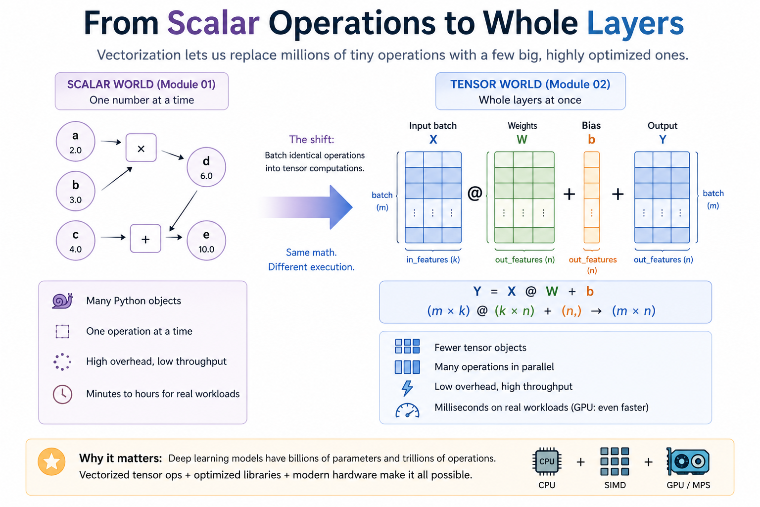
Scalar World (Module 01) vs Tensor World (Module 02): batching scalar operations into tensor ops to reduce overhead and exploit SIMD/GPU parallelism.

In Module 01, every number was its own Python object; one operation at a time, high overhead, low throughput. In Module 02, identical operations across an entire input batch are bundled into a single tensor op that compiles to vectorized native code. Same math, very different execution — and it's the only reason real deep learning is computationally feasible.

Before you start¶

Review 00-prerequisite-review for matrix basics, and 01-autodiff for autodiff mechanics
Review [[PyTorch Primer]] if any of the PyTorch code feels unfamiliar or confusing

Where this fits in¶

The Module 01 autodiff engine works on individual scalars wrapped in Value objects. That's pedagogically beautiful — every node is legible. But it's hopeless for real neural networks. A small MLP on MNIST has thousands of parameters; per-Python-object overhead would make even one forward pass take minutes. A real LLM has hundreds of billions of parameters. Per-scalar Python is not just slow — it's the wrong shape of computation entirely.

The fix is vectorization: stop treating each number as its own object, batch identical operations into bulk array ops, and let optimized native code (NumPy's BLAS, PyTorch's MPS kernels) execute them at near-peak hardware throughput. Modern hardware does many arithmetic operations per clock cycle when fed contiguous data. Vectorized code uses that capacity; per-scalar Python wastes it by a factor of thousands.

The dominant operation in deep learning is matrix multiplication. Linear layers are matmul. Attention is a sequence of matmuls. Embedding lookups are an indexing-then-matmul pattern. Convolutions can be expressed as matmuls. The reason GPUs (and Apple Silicon's MPS) matter for ML is that their architectures are specifically optimized for the bandwidth-and-throughput pattern of large matmuls. Understanding matmul — its math, its memory access pattern, the cost difference between implementations — is the single most important step in seeing why hardware matters.

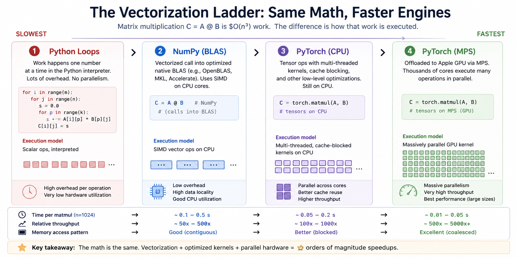The vectorization ladder: Python loops → NumPy (BLAS) → PyTorch CPU → PyTorch MPS, with each rung roughly an order of magnitude faster than the last. Each step up the ladder is roughly an order of magnitude faster than the one below it. Modern deep learning is feasible only because all four rungs exist. trying to train anything serious from rung 1 alone would take years per epoch.

The big idea¶

A tensor is just a multi-dimensional array of numbers. A scalar is 0-D, a vector is 1-D, a matrix is 2-D, a batch of matrices is 3-D, etc. Tensors have a shape (a tuple of dimension sizes) and a dtype (the numeric type of each element).

Two ideas dominate tensor-based numerical code:

1. Matmul. The matrix product C = A @ B where A has shape (m, k) and B has shape (k, n) produces C with shape (m, n). Each entry C[i, j] = sum over p of A[i, p] * B[p, j]. Naively this is m * n * k multiplies and adds — a triple loop. In practice it's the most heavily optimized routine in numerical computing, with vendor-tuned implementations exploiting cache hierarchy, SIMD, and parallelism.

      A          B            C
   (m × k)  @  (k × n)   =  (m × n)
         ↑     ↑
         └─────┘
        inner dims must match;
        they collapse via summation.
        outer dims (m and n) survive.

Matrix Mult Matmul broken down to its atoms. The triple-loop implementation in Exercise 1 just enumerates this directly. Vendor BLAS does the same operation in a fundamentally different way (cache blocking, SIMD, parallelism), but the math is identical.

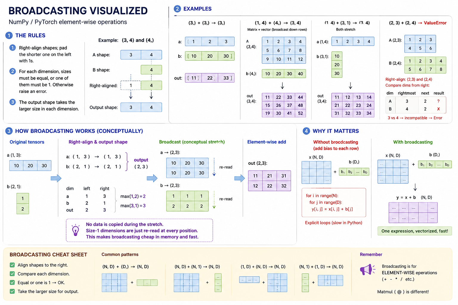
2. Broadcasting. When two tensors with different but compatible shapes are combined element-wise, smaller dimensions are implicitly stretched without copying memory. The standard rules (NumPy and PyTorch use the same):

Right-align the two shapes; pad the shorter one on the left with 1s.
For each dimension, the two sizes must be equal, or one of them must be 1. Otherwise raise an error.
The output shape takes the larger of the two sizes in each dimension.

Examples:

(3,)     + (3,)     -> (3,)         # straightforward
(3, 4)   + (4,)     -> (3, 4)       # vector broadcasts down rows
(1, 4)   + (3, 1)   -> (3, 4)       # both stretch
(2, 3)   + (2, 4)   -> ValueError   # incompatible

Without broadcasting, "add this bias vector to every row of this matrix" requires an explicit loop. With it, you write x + b and it does the right thing.

The trickiest case is the two-way stretch — (1, 3) + (2, 1) — where neither input matches the output shape on its own:

    a = [10  20  30]              shape (1, 3)

    b = [1]                       shape (2, 1)
        [2]

  Both inputs are conceptually "stretched" to the output shape (2, 3):

    a → [10  20  30]              b → [1  1  1]
        [10  20  30]                  [2  2  2]

  Then add element-wise:

      [11  21  31]                 shape (2, 3)
      [12  22  32]

Broadcasting Illustrated Broadcasting is just a simple (and efficient) way to "stretch" shapes so they can be added or multiplied with other shapes of different dimensions

No memory is actually copied during the stretch — the size-1 dimension is just re-read at every position. This is what makes broadcasting cheap.

These two ideas — matmul and broadcasting — together cover an enormous fraction of what neural network code does. Master them and the rest of the course is mostly composition.

Concepts to internalize¶

Tensor = shape + dtype + buffer. A tensor is a contiguous (or strided) block of numbers, plus metadata describing its dimensions.
The matmul shape rule. (m, k) @ (k, n) = (m, n). The inner dimensions agree and collapse.
Why naive matmul is slow. O(n³) operations × per-element Python overhead = unusable. Vectorized matmul is O(n³) operations executed near-peak on the underlying hardware.
Broadcasting rules. Right-align, 1-or-equal, output is element-wise max. Unequal-and-not-1 → error.
Numerical stability of softmax. exp(x_i) overflows for x_i ≳ 88 in float32. Subtract the max along the softmax axis before exponentiating; the result is mathematically identical (softmax is shift-invariant) but stays in floating-point range.
Always know your shapes. Annotate them in comments or docstrings, especially at function boundaries. Most deep learning bugs are silent shape bugs — code that runs and produces wrong numbers because broadcasting masked an error.

What you'll build¶

Package: g2c/tensors/

`matmul.py`¶

matmul_loops(A: list[list[float]], B: list[list[float]]) -> list[list[float]]
matmul_numpy(A: np.ndarray, B: np.ndarray) -> np.ndarray
matmul_torch(A: torch.Tensor, B: torch.Tensor) -> torch.Tensor

All three implement the same operation. The first uses Python loops only. The second uses NumPy. The third uses PyTorch (and respects whatever device the input tensors are on, so it can run on MPS just by passing MPS tensors).

`broadcasting.py`¶

broadcast_shapes(shape_a: tuple[int, ...], shape_b: tuple[int, ...]) -> tuple[int, ...]

class TinyArray:
    data: list[float]
    shape: tuple[int, ...]
    def __add__(self, other: TinyArray) -> TinyArray
    def __mul__(self, other: TinyArray) -> TinyArray

A toy array class supporting NumPy-style broadcasting in element-wise add and multiply. Storage is a flat Python list; broadcasting is implemented entirely in pure Python so that the rules are visible.

`forward.py`¶

linear(x: torch.Tensor, W: torch.Tensor, b: torch.Tensor) -> torch.Tensor
softmax(x: torch.Tensor, dim: int = -1) -> torch.Tensor

A linear layer (y = x @ W + b) and a numerically stable softmax. Together they form the forward pass of a single-layer classifier.

How to run the tests¶

A pytest suite is in tests/test_tensors.py. Initial state: a small number of construction/repr tests pass; the rest fail informatively until you implement.

source .venv/bin/activate

pytest tests/test_tensors.py             # run all module-02 tests
pytest tests/test_tensors.py -x          # stop at first failure
pytest tests/test_tensors.py -k matmul   # only matmul tests
pytest tests/test_tensors.py -v          # verbose

Exercises¶

To launch the exercise notebook run:

./noteboosh.sh 02

If at any point you want to archive the work in your current notebook and restart fresh:

./noteboosh.sh --fresh 02

The notebook carries the exact tables, arrays and questions; this page lists the exercise arc.

Shape tracing. Predict valid and invalid matmul / broadcast shapes.
Manual matmul. Compute a small matrix product and verify it with your implementations.
Benchmark and interpret matmul. Compare loop, NumPy, torch CPU, and torch MPS performance.
Broadcasting predictions. Predict which axes stretch, then verify with TinyArray.
Softmax stability. Explain overflow and why subtracting the max preserves probabilities.
Classifier forward pass. Implement a linear + softmax forward pass with explicit shape annotations.

Pitfalls to expect¶

Off-by-one in the matmul loop. The standard order is for i in range(m): for j in range(n): for p in range(k): C[i][j] += A[i][p] * B[p][j]. Mixing up the inner index breaks correctness silently — always test against NumPy.
Forgetting to subtract the max in softmax. Works fine on small inputs; produces NaN on real-world logits because exp(50.0) overflows float32. The shift-invariance test in the suite catches this.
Broadcasting edge cases. (0,) shapes, scalar inputs (shape ()), single-element dims that need to align across many positions. The test suite covers the common patterns; if a test fails, the failing case is your guide.
Right-aligning the wrong way. Broadcasting aligns shapes by their last (right-most) dimension. A common mistake is to align by the first. Pad on the left with 1s, not the right.
Forgetting to consult .shape. Most "this works but the numbers are wrong" bugs are silent shape mismatches that broadcasting masked. When a test fails, print shapes first.
Using torch.nn.Linear. Don't. The point is to write the matmul + bias yourself with explicit shape discipline.

M-series notes¶

This is the first module that uses Apple Silicon GPU acceleration. The setup script's smoke test already verified MPS is available. For the benchmarks:

Expect MPS matmul to be roughly an order of magnitude faster than torch CPU on large sizes (≥512), with a smaller advantage on small sizes where kernel launch overhead dominates.
A few PyTorch ops still fall back to CPU on MPS even though MPS is selected as the device. For matmul this is not an issue, but if you experiment with other ops you may see warnings — they're informational, not errors.
The first MPS op of a session has a one-time JIT compilation cost. Do a warm-up call before timing.

For the Python loop benchmark: stop at size 512 or 1024 unless you want to wait. The growth is genuinely cubic, and 2048³ Python operations is on the order of an hour.

Reading¶

Primary:

Karpathy, "Neural Networks: Zero to Hero" lectures 2–3. Gets you fluent with the tensor/broadcasting mental model in PyTorch.
PyTorch broadcasting docs. https://pytorch.org/docs/stable/notes/broadcasting.html — the canonical specification of the rules you're implementing.
NumPy broadcasting docs. https://numpy.org/doc/stable/user/basics.broadcasting.html — same rules, slightly different phrasing; useful to read both.

Secondary:

Parr & Howard, "The Matrix Calculus You Need For Deep Learning." Free online. Excellent for solidifying matrix-shape intuition.
Smith, "From Python to NumPy." Free online book on vectorization patterns. Especially the chapter on broadcasting examples.

Optional:

Goto & Van de Geijn, "Anatomy of High-Performance Matrix Multiplication." Why a real BLAS implementation is far faster than your triple loop. Skim if curious.

Deliverable checklist¶

g2c/tensors/matmul.py: all three matmul functions implemented and tests passing
g2c/tensors/broadcasting.py: broadcast_shapes + TinyArray.__add__ + TinyArray.__mul__ passing
g2c/tensors/forward.py: linear and numerically stable softmax passing
notebooks/solutions/02-tensors.ipynb: log-log timing plot across implementations and sizes, including MPS
notebooks/solutions/02-tensors.ipynb: a one-layer classifier forward pass with shape annotations
You can explain, out loud, why the Python-loop matmul falls so far behind NumPy, and what would need to change in your code to close the gap