Module 09 — The transformer block¶

Question this module answers: How do we compose attention and "thinking"?

Transformers are layers of blocks. Each block is an attention sublayer and a normal neural network sublayer. Once you have this block, scaling up is just "stack N of these and add embeddings" + a final unembedding head. The rest of the lesson page is unpacking why each one is where it is.

Before you start¶

Review
- 08-multi-head-attention
- [[PyTorch Primer]] if any PyTorch code feels unfamiliar or confusing
Finish
- g2c/nn (03-nn)
- g2c/embeddings (05-embeddings)
- g2c/attention (08-multi-head-attention and 07-attention)

Where this fits in¶

After Module 08, you have multi-head attention as a standalone mechanism — a learnable mixing operation that lets every position consult every other. But attention alone doesn't support multiple layers, which is the core of deep learning. Attention alone is insufficient at scale. This module shows us an architecture that allows us to stack attention.

The big idea¶

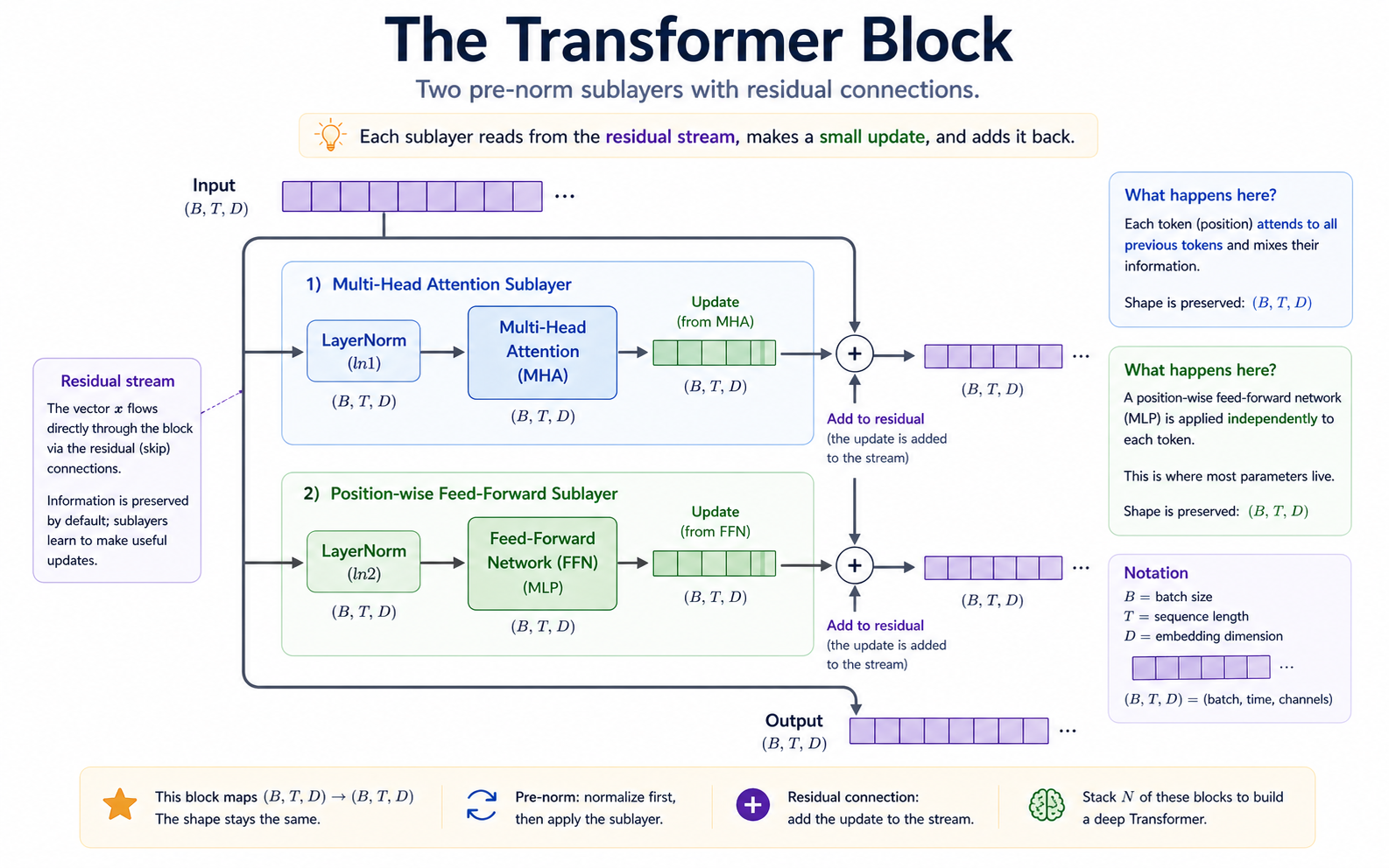
A transformer is attention embedded inside a specific architectural sandwich that makes it trainable at depth. The building block of the transformer is the block. Once you have it, scaling up is "use a larger D, larger T, more blocks."

  ┌─ Multi-head attention sublayer ─────┐
  │                                     │
  x ──► LayerNorm ──► MHA ──► + ──┐
  │                               │
  └──── residual connection ──────┘
                                  │
  ┌─ Feed-forward sublayer ───────┘─────┐
  │                                     │
  x ──► LayerNorm ──► FFN ──► + ──┐
  │                               │
  └──── residual connection ──────┘

Three new ideas wrap around the attention you already have:

Layer normalization keeps activations in a numerically sane range as they flow through the network. Without it, activations can blow up or collapse — and gradients along with them.
Residual connections turn the network into a refinement pipeline rather than a transformation pipeline. Without residuals, deep transformers don't train.
The position-wise feed-forward network gives the model a way to do non-attention computation per position — a per-token MLP applied to whatever attention pulled in. V

These mechanisms combine into the full pipeline of one block. With all the reshape-free arithmetic written out:

       (B, T, D)              ┌────────────────────┐
   x ─┬─► LayerNorm ──► MHA ──► +
      │                       ▲
      └──── residual ─────────┘
                              │
                              ▼
                       (B, T, D)
                              │
                              ├──► LayerNorm ──► FFN ──► +
                              │                          ▲
                              └──── residual ────────────┘
                                                         │
                                                         ▼
                                                  (B, T, D)

Two sublayers. Each sublayer is "normalize → transform → add to residual." The full block in code is exactly this:

def forward(self, x):
    x = x + self.attn(self.ln1(x))     # attention sublayer
    x = x + self.ffn(self.ln2(x))      # FFN sublayer
    return x

Everything important about the transformer architecture is encoded in those two lines.

Feed forward network¶

We covered attention in the past two modules. The second half of the transformer block is the feed-forward network (FFN). The FFN is just a 1-hidden layer MLP, like the ones we trained in Module 3. It uses a slightly version of ReLU (GELU) as the activation layer:

  FFN(x_t)  =  W_2 · GELU(W_1 · x_t + b_1) + b_2     for each position t

The most important thing to keep in mind is that the FFN is per position. There is no mixing between the token positions. The FFN is the "compute" half of the block, attention is the "communication" half. Position t and position s see the same W_1, W_2 but process their own x_t, x_s independently.

In practice, the convetion is to set hidden_dim = 4 × embedding_dim . The complete intermediate projection gives the GELU activation layer room to carve out nonlinear features. Because of this most of the parameters in a transformer actually live in the FFN, not the attention heads.

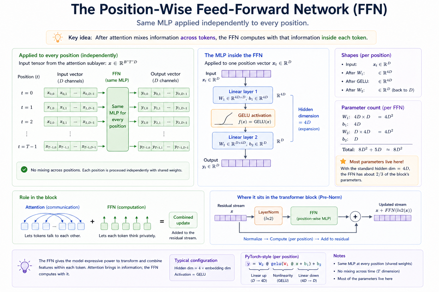*The FFN is the "compute" half of the block. Attention mixes information, the FFN is what the model does with that mixture.

Residual connections¶

Residual connections are how we "stack" layers of transformer blocks. Without residual connections, transformers deeper than a handful of layers fail to train. With them, training scales to hundreds of layers. The intuition has two complementary flavors:

Residual-stream view. Think of x as a "communication bus" through the layers of the network. Each sublayer reads the bus, produces an update, and writes the update back onto the bus. Sublayers are contributions to the residual stream rather than replacements of it. The model's "no-op behavior" is to pass information through. Sublayers therefore specialize to make targeted edits.

Gradient-flow view. During backprop, ∂loss/∂x at the input depends on the chain of partial derivatives through every sublayer. In a non-residual network, that chain multiplies through every sublayer's Jacobian; if those Jacobians have spectral norm < 1 , the gradient shrinks exponentially with depth — vanishing gradients. By contrast the residual approach turns the chain into 1 + ∂sublayer/∂x at each step. The 1 term ensures gradients flow through the residual path even when ∂sublayer/∂x ≈ 0. Gradients no longer vanish completely.

  Without residuals:        With residuals:

   x  ─► f1 ─► f2 ─► f3       x  ─┬─► f1 ─► +  ─┬─► f2 ─► +  ─┬─► f3 ─► +
                                 │             │             │
                                 └────────────┘             │
                                               └────────────┘
                                                             └──── ...

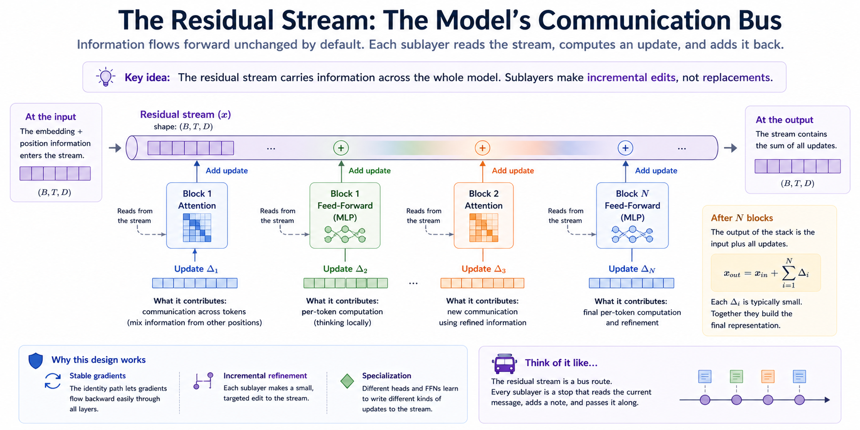*Sublayers make incremental edits, not replacements. This is the property that makes deep transformers trainable (gradient-flow view)

LayerNorm¶

LayerNorm is what keeps the scale of the residual stream bounded as we move between layers. Without it, after a few blocks the residual may accumulate so many unnormalized sublayer outputs that its magnitude diverges, and training stop works.

  LayerNorm(x):
      mean = x.mean(dim=-1)        # over channels, NOT batch
      var  = x.var(dim=-1)         # over channels, NOT batch
      x_hat = (x - mean) / sqrt(var + ε)
      return γ * x_hat + β

Three properties of LayerNorm are worth internalizing:

It normalizes per-token. For input shape (B, T, D), LayerNorm pools statistics over the D axis only. Each (B, T) position is normalized independently. That's why batch size doesn't affect the output, and train and inference behavior are identical.
The learned affine γ, β is the escape hatch. Pure standardization would lock every output's mean and variance to 0 and 1, which constrains the next layer. The affine parameters let the model freely choose any mean and variance, but initialized to start at (1, 0)
The ε in the sqrt is structural, not cosmetic. A near-constant input has near-zero variance, and dividing by sqrt(0) produces NaN. ε = 1e-5 keeps the divisor away from zero with negligible effect on normal inputs.

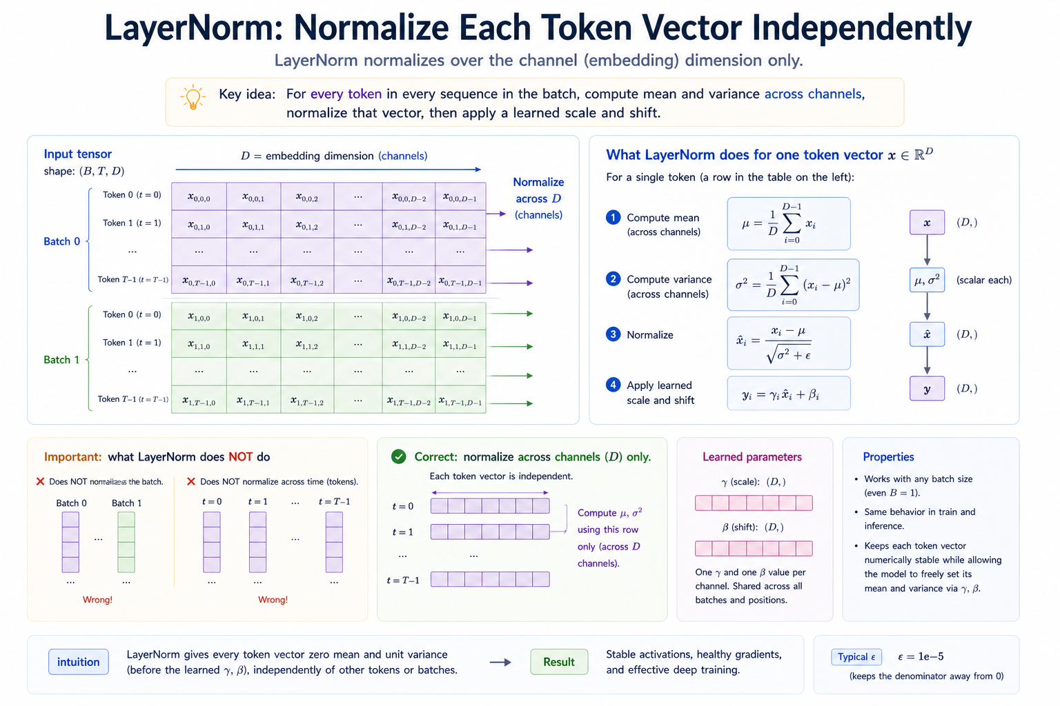LayerNorm normalizes each token vector independently across channels, and learns scale/shfit. The key distinction from BatchNorm is "pool over channels, not over the batch."

One minor note for how LayerNorm is applied. The original 2017 transformer (Vaswani et al.) used post-norm:

  Post-norm:    x = LN(x + sublayer(x))

The modern transformer uses pre-norm

  Pre-norm:     x = x + sublayer(LN(x))

The difference is one of operation order, but it's load-bearing for numerical stability during training and preventing vanishing gradients. Xiong (2020) go into more details on the reasons why. For this course it's sufficient to simply remember to always normalize first then apply the sublayer, rather than appying the sublayer first then normalizing.

  Pre-norm pipeline (this module):

     x ──┬─► LN ──► sublayer ──► +
         │                       ▲
         └─── residual stream ───┘    ← residual flows past LN

  Post-norm pipeline (Vaswani 2017):

     x ──┬─► sublayer ──► + ──► LN
         │               ▲
         └── residual ───┘             ← residual flows through LN

Tied embeddings¶

The final part of our transformer stack are tied embeddings. This just means the model uses the same token embeddings at the initial input and final output. Transformers have embedding weights to convert tokens to vectors at input, and unembedding weights to convert vectors back to tokens at the the ouput. With tied embeddings we make both sides same matrix.

  TokenEmbedding.weight    (V, D)   ◄── input end of the tie
        │
        ▼
   + positional
        │
        ▼
   N × Block
        │
        ▼
   final LayerNorm
        │
        ▼
   logits = x @ token_embed.weight.T + head_bias    ◄── output end

The two roles are asking the same question. The input table is "the vector that represents token v." The output projection is "the direction that scores token v." Those are nearly the same object. In practice, training pulls them toward each other anyway. Tying just commits to the answer up front.

Tying is useful because it conserves parameters, reducing compute and data requirements. The accounting:

  Untied:   V*D (input) + V*D (output) + V (output bias)  =  2*V*D + V
  Tied:     V*D (shared) + V (output bias)                =    V*D + V
  Saving:   V*D parameters

The full TransformerLM¶

TransformerLM is the minimal viable language model: embed, refine through N blocks, normalize, and unembed.

  token_ids  ──► TokenEmbedding   ──┐
                                     ├──► +  ──► N × Block ──► LayerNorm ──► unembed ──► logits
  positions  ──► PositionalEmbed  ──┘

  shapes:
    token_ids   (B, T)
    tok         (B, T, D)
    pos         (T, D)         broadcasts to (B, T, D)
    x           (B, T, D)      after every block
    logits      (B, T, V)

Two details worth pinning down:

One logit per position. Output is (B, T, V), not (B, V). Position t's logit is the prediction for what comes at position t+1. At training time, you compute cross-entropy at every position in parallel — vastly more efficient than the one-position-per-step training of the Module 06 MLP.
The final LayerNorm before unembedding. Modern transformers add this; the original 2017 paper didn't. Without it, the residual stream's scale at the output is unbounded and the unembedding's logits can drift arbitrarily large or small. A small, cheap correction.

Concepts to internalize¶

The transformer block is two sublayers, each pre-normalized and residually wrapped. That's the entire architectural delta from pure attention.
The residual stream is the model's "communication bus." Sublayers add contributions to it; they don't replace it.
LayerNorm normalizes over the channel dim only. Each (B, T) position is normalized independently — no cross-position or cross-batch pooling.
Pre-norm is the modern default. Trains stably at depth without warmup; post-norm needs warmup or diverges.
The FFN is per-position with a 4× hidden expansion. Most of a transformer's parameters live here.
Stacking blocks is straightforward. for block in self.blocks: x = block(x). The architecture has no positional encoding between blocks, no cross-block coupling, no per-block parameters that depend on layer index. Each block is a self-contained refinement step.
Tied embeddings: one set of token weights is used for both input and output. Reflects that "vector for token v" and "direction that scores token v" are nearly the same object.
TransformerLM outputs (B, T, V) logits. One next-token prediction per position, computed in parallel during training.

What we don't cover¶

Dropout. Used by Vaswani et al. and many follow-ups for regularization; not strictly necessary at the small scales we'll train, and it adds a training/eval mode distinction that our minimal Module base class doesn't model. Out of scope.
RMSNorm (used by Llama and other modern transformers). A simplified LayerNorm without the mean-subtraction step. Equivalent in practice but conceptually a small variation; we use vanilla LN.
Mixed precision, gradient checkpointing, fused ops. Module 10 pretraining concerns, not architecture concerns.

What you'll build¶

Package: g2c/transformer/

class LayerNorm(Module):
    embedding_dim: int
    eps: float
    gamma: torch.Tensor                  # (D,)
    beta: torch.Tensor                   # (D,)

    def parameters(self): ...                                   # implemented
    def forward(self, x): ...                                   # SCAFFOLDED

class FeedForward(Module):
    embedding_dim: int
    hidden_dim: int                      # default: 4 * embedding_dim
    fc1: Linear                          # (D, hidden_dim)
    fc2: Linear                          # (hidden_dim, D)

    def parameters(self): ...                                   # implemented
    def forward(self, x): ...                                   # SCAFFOLDED

class Block(Module):
    embedding_dim: int
    num_heads: int
    hidden_dim: int
    causal: bool
    ln1: LayerNorm
    attn: MultiHeadAttention
    ln2: LayerNorm
    ffn: FeedForward

    def parameters(self): ...                                                            # implemented
    def forward(self, x): ...                                                            # SCAFFOLDED

class TransformerLM(Module):
    vocab_size: int
    embedding_dim: int
    num_layers: int
    num_heads: int
    max_seq_len: int
    hidden_dim: int
    token_embed: TokenEmbedding
    pos_embed: LearnedPositionalEmbedding
    blocks: list[Block]
    ln_final: LayerNorm
    head: Linear

    def parameters(self): ...                                                                                    # implemented
    def forward(self, token_ids): ...                                                                            # SCAFFOLDED

Total scaffolded code: roughly 20 lines split across four forward methods. Most of the lesson is in which lines and in what order — the math is unsubtle once you've internalized the structure.

How to run the tests¶

Tests live in tests/test_transformer.py. Initial state: 22 passed (all the construction, parameter-count, and init-value checks), 22 failed.

source .venv/bin/activate

pytest tests/test_transformer.py             # run all module-09 tests
pytest tests/test_transformer.py -x          # stop at first failure (recommended)
pytest tests/test_transformer.py -k layer_norm   # only LayerNorm tests
pytest tests/test_transformer.py -k block    # only Block tests
pytest tests/test_transformer.py -v          # verbose

Exercises¶

To launch the exercise notebook run:

./noteboosh.sh 09

If at any point you want to archive the work in your current notebook and restart fresh:

./noteboosh.sh --fresh 09

The notebook contains the ablations and plotting scaffolds.

Post-norm ablation. Compare post-norm and pre-norm training curves.
Remove residuals. Watch deeper blocks stop training without the residual highway.
Remove layer norm. Observe unstable activation scale and loss behavior.
Depth vs width. Compare similarly sized transformer configurations.
Parameter-count sanity check. Derive and verify the full TransformerLM parameter count.

Pitfalls to expect¶

LayerNorm over the wrong dim. Pooling statistics over the batch dim (BatchNorm-style) or over the sequence dim instead of the channel dim. Symptom: training works but is unusually slow; batch size matters in surprising ways.
unbiased=True in the variance. Divides by N - 1 instead of N — the sample variance instead of the population variance. Off by a factor of D / (D - 1) from the standard implementation. Hard to notice; impossible to debug.
Forgetting eps. A constant-along-channel input has zero variance and your normalized vector is 0 / sqrt(0) = NaN. The test test_layer_norm_handles_constant_input catches this.
Post-norm by accident. Writing x = self.ln1(x + self.attn(x)) instead of x = x + self.attn(self.ln1(x)). The shape is the same, the test for output shape passes, but training is dramatically less stable.
Forgetting the residual. Writing x = self.attn(self.ln1(x)) instead of x = x + self.attn(self.ln1(x)). The model becomes untrainable past 2-3 layers.
Sharing one LayerNorm between sublayers. Reusing self.ln1 for both the attention and FFN sublayers instead of having a separate self.ln2. Doesn't crash, but reduces expressiveness — the FFN loses its independent scale/shift.
Forgetting the final LayerNorm in TransformerLM. A common oversight; the original 2017 transformer didn't have one, but every modern transformer does. Without it, the head's logits can drift arbitrarily large or small as training progresses.
Wiring pos_embed outside the broadcast. pos = self.pos_embed(T) has shape (T, D). Adding it to tok of shape (B, T, D) works via broadcasting — but if you accidentally write pos.unsqueeze(0) you get (1, T, D) which also broadcasts but hints at a confused mental model. Both work; one is cleaner.
for block in self.blocks: x = block(x) is sequential — do NOT parallelize it. Block i reads block i-1's output. Trying to run them concurrently misunderstands the architecture (this is a recurring beginner instinct; the transformer is parallel within a block, sequential across blocks).

M-series notes¶

This module is still light on compute.

Exercise 1's pre-norm vs post-norm comparison at num_layers = 6, D = 64, T = 32 is a few minutes per run on CPU; comfortable on MPS.
Exercise 2's strip-residuals study at num_layers = 8 is the first configuration big enough that MPS starts paying off — about 2× over CPU at this size.
Exercise 4's parameter-budget comparison is also CPU-comfortable but a good place to start using MPS as practice for Module 10.

The notebook uses MPS by default for training. switch to device="cpu" if you want to compare explicitly.

Reading¶

Primary:

Vaswani et al., "Attention Is All You Need" (2017), §3. The block structure is defined in figure 1 and §3.1. Note that the 2017 paper uses post-norm; if you read it as an intro, mentally translate "norm after sublayer" into "norm before sublayer" because every modern reading you'll do uses pre-norm.
Ba, Kiros, Hinton, "Layer Normalization" (2016). The original LayerNorm paper. Short, direct, and worth reading once for the motivation contrast against batch normalization.
Karpathy, "Let's build GPT: from scratch, in code, spelled out" (YouTube). The block-assembly section walks through this same composition step by step.

Secondary:

Xiong et al., "On Layer Normalization in the Transformer Architecture" (2020). The paper that established that pre-norm trains more stably than post-norm. Argues theoretically and empirically; the figure showing post-norm needing warmup and pre-norm not is the headline.
Anthropic, "A Mathematical Framework for Transformer Circuits" (2021), introductory sections. Frames the residual stream as a communication bus that every sublayer reads from and writes to. The conceptual model that underlies most of mechanistic-interpretability research.
He et al., "Deep Residual Learning for Image Recognition" (2015). The original residual-connection paper, in computer vision. Predates the transformer by two years; the same insight ("training deep networks fails without identity shortcuts") drives both architectures.

Optional:

Zhang & Sennrich, "Root Mean Square Layer Normalization" (2019). RMSNorm — a simplified LN that drops the mean-subtraction step. Used by Llama and many recent transformers; a few percent faster, no quality loss in practice.
Press et al., "Using the Output Embedding to Improve Language Models" (2017). The case for tied input/output embeddings — saves parameters at no quality cost. Our TransformerLM uses tied embeddings; this is the paper that established the technique.

Deliverable checklist¶

All tests in tests/test_transformer.py pass.
Notebook: notebooks/clean/09-transformer-block.ipynb. Work through pre-vs-post norm, residual ablations, shape checks, and parameter-budget sanity checks.
You can explain — out loud, without notes — why residual connections make deep transformers trainable, in both the gradient-flow and residual-stream framings.
You can explain — out loud, without notes — what LayerNorm normalizes over, and why batch size doesn't affect its output.
You can explain — out loud, without notes — the difference between pre-norm and post-norm, and why pre-norm is the modern default.