Module 07 — Self-attention

Question this module answers: How can tokens communicate?

The same pipeline runs at every position in parallel, with the only per-position difference being which Q vector poses the question. Most of the rest of this lesson page is unpacking the "why" behind the pipeline. This week is the hinge of the course — everything from here through the transformer block is variations on what you build this week.

---

Before you start

• Review 06-language-models for the next-token-prediction setup that attention extends
• Finish g2c/nn from 03-nn, g2c/embeddings from 05-embeddings, and g2c/tokenizer from 04-tokenizer — exercise 3 trains a tiny LM end-to-end and needs all three

---

Where this fits in

With Module 06 you have a MLP language model that predicts next token from a fixed-length window of preceding tokens. It works, but has two ceilings that don't go away:

1. Fixed context. The MLP has one set of weights per position in its concat. To extend the context length you have to grow the weight matrix. Doubling the context doubles the parameter count.
2. No inter-token communication. The MLP can attend to "what's at each position" but it can't attend to "the relationship between this position and that position." Embeddings are pooled by concatenation and never get to look at each other.

Self-attention solves both at once. It's a parameter-efficient, sequence-length-agnostic, learnable mixing rule that lets every position consult every other position. The Q, K, V projections cost a fixed O(D²) parameters regardless of sequence length, and the mixing weights are computed dynamically from the data — no fixed slot per position.

The conceptual move is roughly the same one calculus took with the limit: we replace a discrete table indexed by position with a continuous similarity-based weighted sum. Once you've built this, the rest of the transformer is plumbing.

The big idea

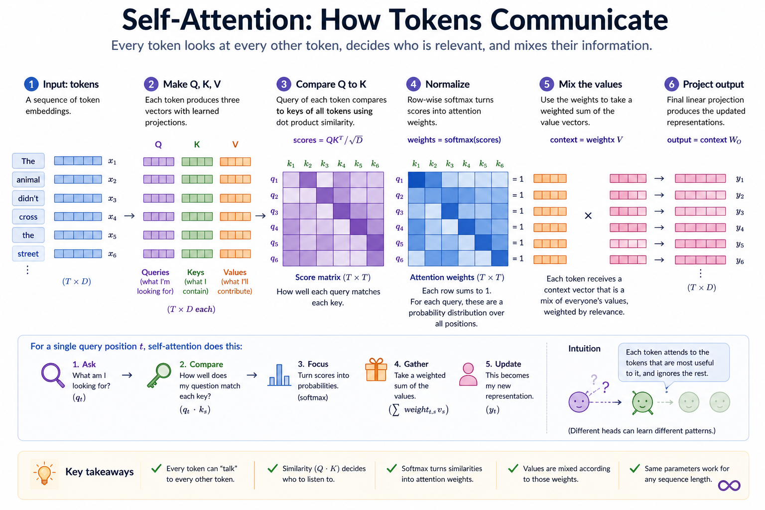
Each token wants to update its own representation based on the rest of the sequence. To do that, it needs three things from every other token:

  Position  t   asks:  "what am I looking for?"        →  query  q_t
  Position  s   says:  "here's what I have on offer"   →  key    k_s
  Position  s   says:  "and here's what I'd contribute" → value  v_s

The "match score" between query t and key s is the dot product q_t · k_s. Big positive means "this is what t was looking for." Apply softmax over s to turn the row of scores into a probability distribution over context positions; use those probabilities as weights to take a weighted sum of v_s. That weighted sum becomes the output at position t.

  Pipeline (single head, no batch dim, sequence length T = 4):

      x  ──┬──► Wq ──► Q  (T, D)
           ├──► Wk ──► K  (T, D)
           └──► Wv ──► V  (T, D)

      scores  =  Q @ K.T  /  sqrt(D)               # (T, T)
                                              ┌──► row-softmax
      apply causal mask (-inf above diagonal) ┘
                                                    ↓
                                              weights (T, T)
                                                    │
                                              weights @ V  (T, D)
                                                    │
                                              Wo  ──►  output (T, D)

The whole module is that diagram, generalized to a batch dim.

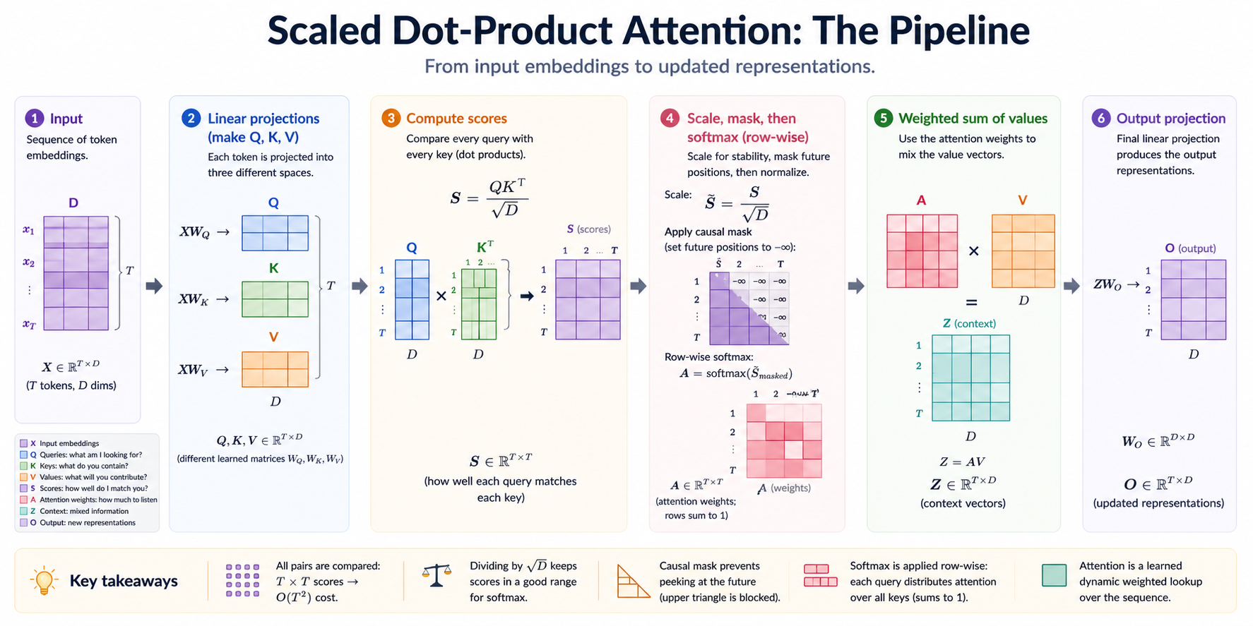Two details worth lingering on: the score matrix is always (T, T) regardless of D — that's the quadratic cost ceiling — and the √D divide before softmax is what keeps the softmax in a non-saturated regime as D grows, which is the most common bug to forget.

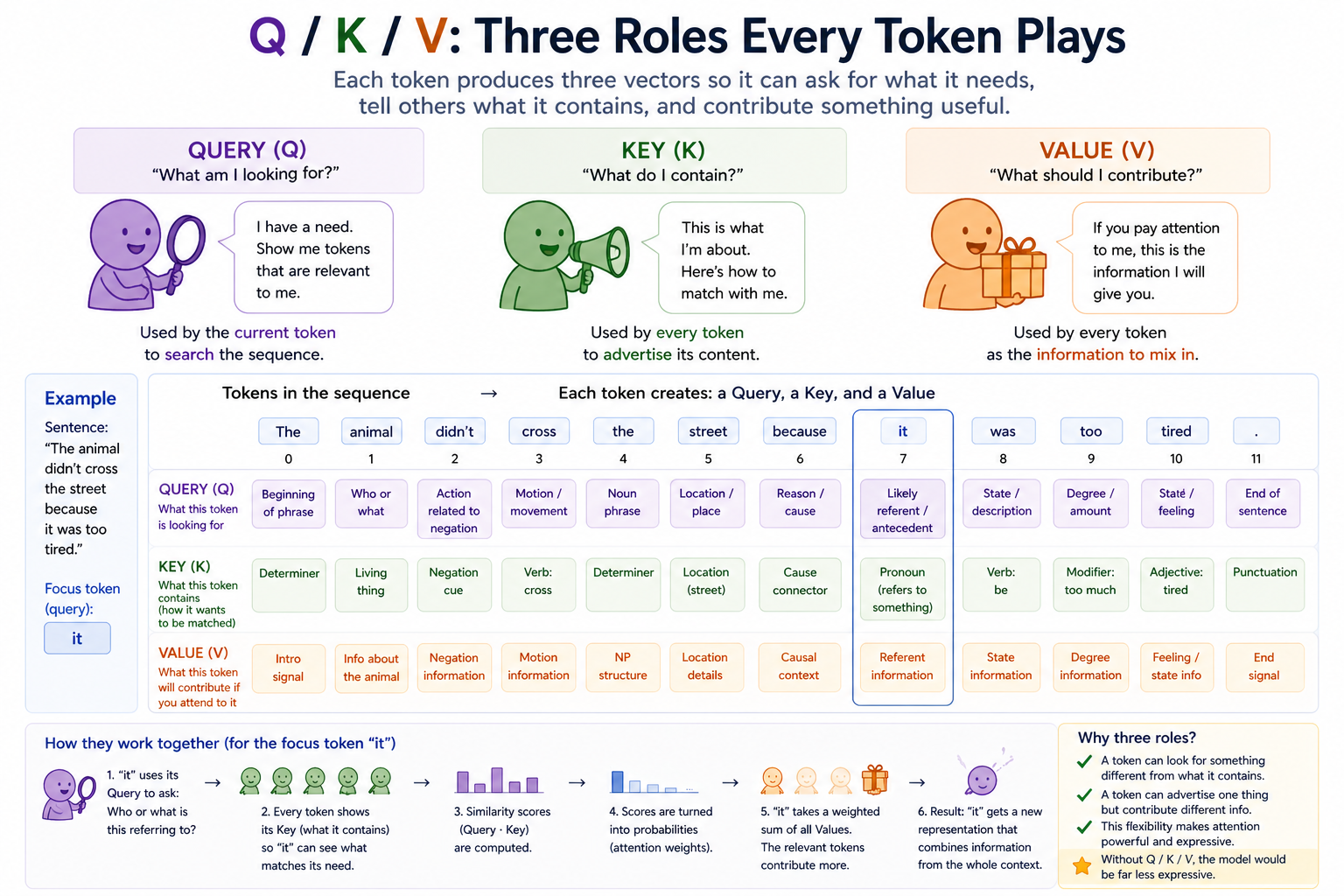
Why Q, K, V are three different projections

In principle you could use the input vectors themselves as queries, keys, and values: q_t = k_t = v_t = x_t. That works mathematically. But it forces "what I'm looking for" and "what I have on offer" and "what I contribute" to all be the same vector. By projecting x through three independent learned matrices, the model can keep these three roles separate — a token can advertise something different in its key than it actually contributes in its value, and ask for something else entirely in its query. Almost all of attention's expressive power comes from this decoupling.

The output projection W_o plays a similar role: it lets the model remap the mixed values back into a representation space that's useful for the next layer. (In single-head attention W_o is mostly ceremonial; in multi-head attention it's where the heads' outputs get combined and is genuinely critical.)

The decoupling is what gives attention its expressive power. With one shared projection ("just use x"), the same vector would have to simultaneously be a question, an advertisement, and a contribution — three jobs that pull in different directions during training. Three separate matrices let each role specialize.

The √D scaling

The scores Q @ K.T are dot products of D-dimensional vectors. If Q and K have unit-variance entries, the variance of each dot product scales as D. As D grows, the scores get larger and more spread out; after softmax, almost all the mass concentrates on a single position and gradients with respect to the rest collapse. This is the same "vanishing gradients in saturated softmax" failure mode you'll see again in Module 09 with deep networks.

Dividing by sqrt(D) re-normalizes the scores to unit variance so the softmax stays in a non-saturated regime regardless of D. It's a one-character change with an outsized effect on training stability — forgetting it is the most common bug in from-scratch attention code.

The causal mask

In a language model, position t's prediction must depend only on positions 0..t. If position t could attend to position t+1, the training objective collapses: the model's "prediction" at position t can just copy the value at position t+1 and get next-token cross-entropy of zero. This is a famously catastrophic bug that silently looks like training success.

The fix is to set scores[t, s] = -inf for all s > t BEFORE the softmax. After softmax those entries become exactly zero — position t literally cannot attend to position s > t because its weight is zero, so the value at s > t cannot leak into the output at t.

  causal_mask(T=5)  (True = blocked)

       s=0   s=1   s=2   s=3   s=4
  t=0  [F     T     T     T     T  ]
  t=1  [F     F     T     T     T  ]
  t=2  [F     F     F     T     T  ]
  t=3  [F     F     F     F     T  ]
  t=4  [F     F     F     F     F  ]

  Diagonal is False — every position can attend to itself.
  Above-diagonal is True — no peeking at the future.

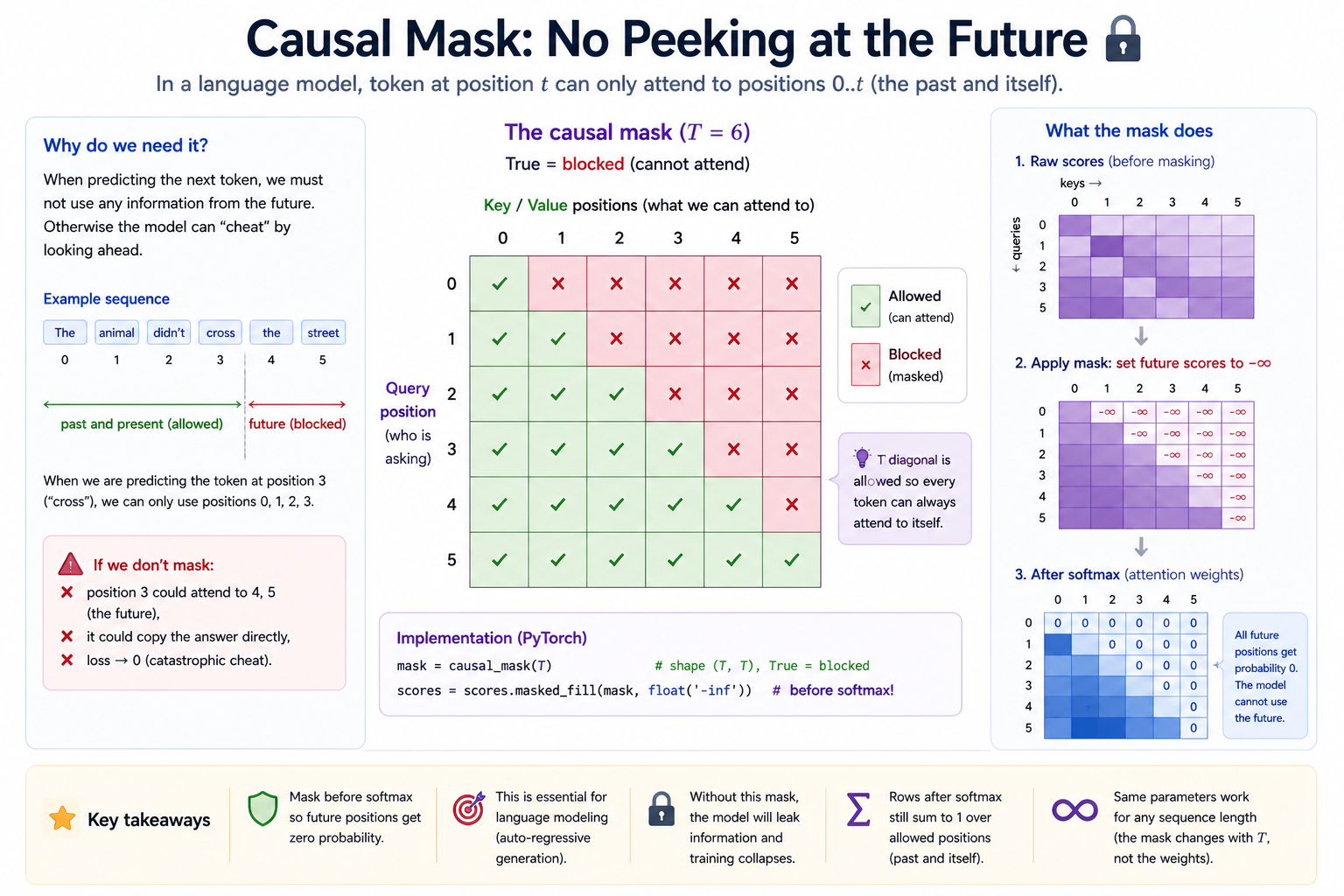The mask is applied BEFORE the softmax so the −∞ scores become exact zeros after exponentiation, not merely small numbers. Setting the post-softmax weights to zero directly would be wrong — the remaining weights wouldn't sum to 1.

The convention "True means blocked" matches masked_fill(mask, value), which fills wherever the mask is True. The causal_mask static method on SelfAttention is implemented for you because it's bookkeeping, not the lesson.

Exercise 3 will have you flip causal=False, train briefly, and watch the loss drop to ~0. That collapse is the visceral signal that the mask is doing real work.

Self-attention is permutation-equivariant

If you shuffle the tokens of a sequence and feed them through a vanilla self-attention layer (with no positional encoding), the output is shuffled the same way. The mechanism has no notion of "position 1 is before position 2" — it only sees similarities between vectors. That's the bag-of-tokens failure mode that motivated positional embeddings in Module 05.

In practice, attention is always preceded by a positional encoding step (sinusoidal, learned, or RoPE) that breaks this symmetry. Module 07 ignores positions because the goal is to study attention itself in isolation; Module 09 wires the two together when assembling the full transformer block.

The quadratic-cost gotcha

The score matrix is (T, T) and grows with the square of the sequence length. For T = 1024 it has a million entries; for T = 32k (a typical chat context length) it has a billion. Self-attention's O(T²) memory and compute is the famous bottleneck that motivates the last decade of efficient-attention research (sparse, linear, FlashAttention, state-space models). Module 07 doesn't try to fix this — but you should feel it. The numbers above are the reason attention can't naively scale to very long contexts.

Concepts to internalize

• Attention is a learnable gather. A weighted sum where the weights depend on the data, not on a fixed position.
• Q, K, V are three projections of the same input. Each plays a different role; the decoupling is where the expressive power comes from.
• Scores are dot products, scaled by 1/√D. Without the scaling, softmax saturates as D grows.
• The causal mask must be applied before softmax. Masking after softmax destroys the row-sum-to-1 property and is the bug everyone introduces at least once.
• Self-attention is sequence-length-agnostic. No fixed-length weights; the same parameters handle any T. This is the structural property that lets transformers generalize across context lengths and is why positional encoding is decoupled from the layer itself.
• Cost is O(T²) in time and memory. Felt as soon as T exceeds a few thousand. Worth feeling now so the efficient-attention literature later makes sense.
• Self-attention is permutation-equivariant on its own. Position must be injected externally (Module 05's job, wired up in Module 09).

---

What you'll build

Package: g2c/attention/ (self_attention.py only)

class SelfAttention(Module):
    embedding_dim: int
    causal: bool
    q_proj: Linear           # (D, D)
    k_proj: Linear           # (D, D)
    v_proj: Linear           # (D, D)
    out_proj: Linear         # (D, D)

    def __init__(self, embedding_dim: int, *, causal: bool = True): ...   # implemented
    def parameters(self) -> Iterable[torch.Tensor]: ...                    # implemented

    @staticmethod
    def causal_mask(seq_len: int, device=None) -> torch.Tensor: ...        # implemented

    def forward(self, x: torch.Tensor) -> torch.Tensor: ...                # SCAFFOLDED
    def attention_weights(self, x: torch.Tensor) -> torch.Tensor: ...      # SCAFFOLDED

Roughly 15 lines of real code split across the two scaffolded methods. The smallest module-by-LOC of the course so far — and arguably the most important one. Every transformer ever trained uses this exact mechanism.

How to run the tests

Tests live in tests/test_attention.py. Initial state: 9 passed (construction + causal_mask), 14 failed.

source .venv/bin/activate

pytest tests/test_attention.py             # run all module-07 tests
pytest tests/test_attention.py -x          # stop at first failure (recommended)
pytest tests/test_attention.py -k forward  # only the forward tests
pytest tests/test_attention.py -v          # verbose

Exercises

To launch the exercise notebook run:

./noteboosh.sh 07

If at any point you want to archive the work in your current notebook and restart fresh:

./noteboosh.sh --fresh 07

The notebook contains the runnable attention visualizations and small training probes.

1. Hand-compute attention. Verify every step of a 3-token self-attention example.
2. Visualize attention. Plot random causal attention on two sentences using the reusable G2CTokenizer at vocab 2048 when available, with a character-tokenizer fallback. The mask should already be visible; training only changes how probability is distributed over allowed past tokens. Then compare with a lightly trained TinyShakespeare probe that uses ShakespeareTokenizer at vocab 2048 when available.
3. Strip-mask experiment. Show how non-causal attention cheats on next-token prediction.
4. Parameter counts. Verify attention parameter count grows with D, not T.
5. Quadratic cost. Time attention as sequence length increases.

Pitfalls to expect

• Forgetting the 1/√D scaling. Training is unstable; loss is noisy and slow to converge. The model can still learn, but the training curve looks bad.

• Softmax along the wrong dim. scores.softmax(dim=-1) is correct — for each query position, normalize over key positions. dim=-2 normalizes over query positions per key, which is a different (and wrong) computation. Symptom: weights don't sum to 1 along rows.

• Mask polarity backwards. causal_mask returns True above the diagonal (the positions to block). If you pass ~mask to masked_fill, you'll mask positions 0..t and let position t attend only to the future — exactly the opposite of what you want.

• Mask AFTER softmax. Setting masked entries to 0 after softmax destroys the row-sums-to-one property; renormalizing afterwards is numerically unstable and not what we want anyway. Always mask before softmax.

• Transposing the wrong dims. K.T would transpose only a 2D tensor; for a 3D (B, T, D) tensor you need K.transpose(-2, -1) to get (B, D, T). The wrong transpose silently produces wrong-sized outputs that throw later in the pipeline.

• Using attention_weights and forward with different code paths. If you compute scores or apply the mask differently in the two methods, the visualization no longer reflects the actual attention pattern used by forward.

• Running attention on un-positioned embeddings and expecting it to learn order. Self-attention is permutation-equivariant — without positional information, "dog bites man" and "man bites dog" produce the same set of output vectors (just permuted).

M-series notes

This module is light on compute.

• The visualization exercise is forward-pass-only on two short sentences. It uses the reusable G2CTokenizer when available, or a character-tokenizer fallback — milliseconds either way.
• The optional TinyShakespeare attention probe uses ShakespeareTokenizer at vocab 2048 when available and caps the training stream at 1,000,000 tokens. It is still a tiny single-layer model, but the larger token stream can take a few minutes depending on hardware.
• Exercise 3's strip-mask experiment is a few hundred training steps on a small corpus with a single attention layer — under a minute on CPU.
• Exercise 5's O(T²) timing demo at T = 4096, D = 128 allocates a 16M-entry (T, T) score tensor — comfortable on a 16GB machine. If you push to T = 16384 it's a 256M-entry tensor (~1GB at fp32); manageable but you'll feel it.

The clean notebook uses experiment_device = "auto" in the strip-mask training helper. CPU is still fine at the default size. If you increase steps, D, or T, the helper will move the model and minibatches to MPS when available.

---

Reading

Primary:

• Vaswani et al., "Attention Is All You Need" (2017), §3.2. The paper that introduced this exact mechanism. Sections 3.2.1 (Scaled Dot-Product Attention) and 3.2.3 (the masking scheme) are the parts you're implementing. The whole paper is short and a must read at least once.
• Karpathy, "Let's build GPT: from scratch, in code, spelled out" (YouTube). The attention section walks through this same construction with PyTorch — different idioms, identical math. The "self-attention block" derivation in particular is excellent.
• Alammar, "The Illustrated Transformer." The classic visual explainer. The Q/K/V geometric intuition is hard to beat.

Secondary:

• Bahdanau, Cho, Bengio, "Neural Machine Translation by Jointly Learning to Align and Translate" (2014). The paper that introduced attention (in an encoder-decoder RNN context, not yet self-attention). Useful for seeing the conceptual move in its original form: a learned weighted-average over encoder states.
• Elhage et al., "A Mathematical Framework for Transformer Circuits" (Anthropic, 2021), introductory sections. A careful re-derivation of attention from a circuits-interpretability angle. Builds intuition for what individual heads learn.

Optional:

• Dao et al., "FlashAttention: Fast and Memory-Efficient Exact Attention with IO-Awareness" (2022). Skim — the algorithm itself is out of scope for this course, but understanding what the bottleneck is and how it gets fixed is part of the intuition for the modern inference stack.

Deliverable checklist

• All tests in tests/test_attention.py pass.
• notebooks/clean/07-attention.ipynb: attention heatmaps for the two "the animal didn't cross the street..." sentences using your attention_weights method.
• Strip-mask experiment: side-by-side training runs of a tiny attention-only LM with causal=True and causal=False. Loss curves saved; the catastrophic collapse with causal=False is visible.
• You can explain — out loud, without notes — why dividing by sqrt(D) is necessary and what specifically goes wrong without it.
• You can explain — out loud, without notes — what a "permutation- equivariant layer" means and why self-attention is one.