Module 14 — Preference tuning (DPO)¶
Question this module answers: Why is the model helpful, polite, or stylistically consistent?
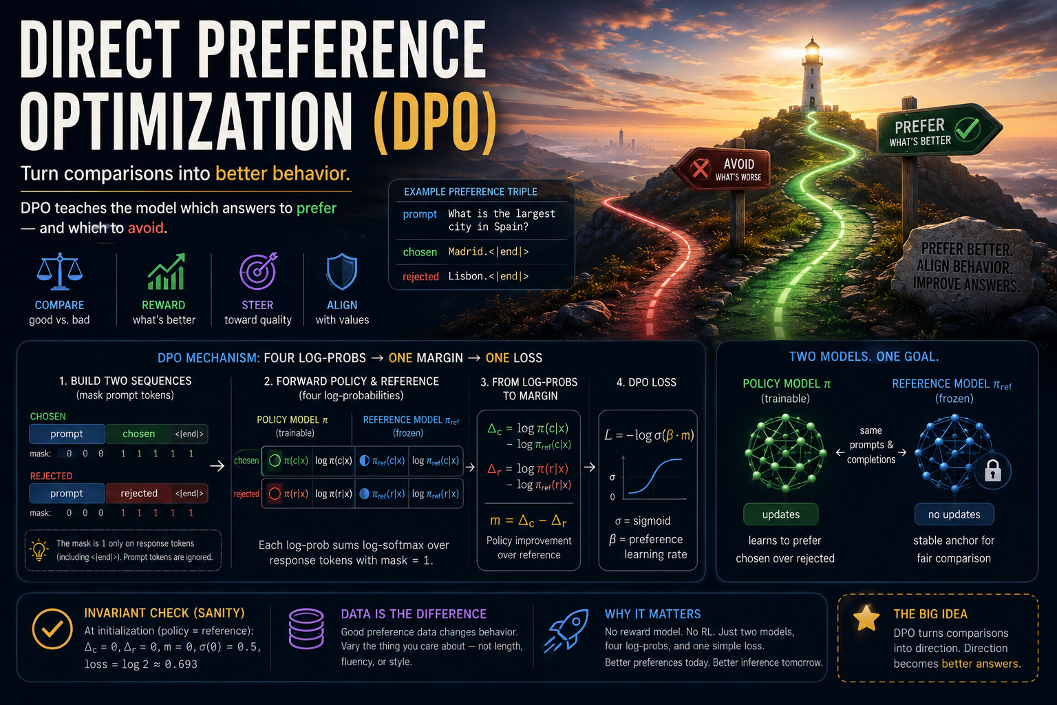
Preference tuning changes the training signal from "imitate this answer" to "prefer this answer over that one." That comparative signal is what DPO turns into a direct loss. Last week we taught the model to format an answer. This week we teach it to prefer one answer over another. Pair up responses, evaluate the preferred choice, and train on those preferences. No new architecture, no reward model. The 50–200 preference pairs are the entire training set. Everything else is plumbing.
Before you start¶
- Review
- 13-sft for the chat template and masking
- PyTorch Primer if any PyTorch code is unfamiliar or confusing
- Finish
g2c/nnfrom 03-nng2c/trainingfrom 03b-training- A post-SFT instruct model from the 13-sft exercise notebook
Where this fits in¶
After Module 13 your SFT'd model produces well-formatted assistant turns:
Confident. Format-perfect. Wrong. Nothing in SFT training penalized this output: unless this exact question appeared in the SFT set with Madrid. as the target, the loss never expressed a preference between one well-formatted city and another. SFT only supplies positive demonstrations — "produce this target" — so its reach ends where the data's coverage ends. The model "knows" the prompt is asking about a Spanish city; it picks city-shaped tokens that pretraining over-represented from the corpus. SFT taught it the shape of the answer; nothing taught it which answer is correct.
SFT was the first layer of post-training in our LLM stack. This week we're exploring DPO, another form of post-training that teaches pairwise preferences. This is more powerful than it appears at first. Many behavioral criteria, including factual accuracy, can be represented by having graders repeatedly pick between two different examples.
SFT is used to post-train the shape of the output response. DPO is used to introduce behavior like helpfulness, honesty, tone, safety, and instruction following — or more precisely, whatever distinctions the preference data actually exhibits; DPO shifts probability toward what the chosen examples share, no more. Because these properties are downstream of having the basic assistant-like shape, DPO comes after SFT in the post-training pipeline.
The nomenclature can be a bit confusing. In almost every case the "base model" that DPO trains over is the SFT model, not the original pretrained model. In this module we'll train DPO on top of the SFT model from Module 13.
The big idea¶
In SFT post-training, we trained on a set of prompt-response examples. The limitation is that this can teach generalized behavior, but is weak at demonstrating specific properties. The model learns "answers should look like this". It doesn't learn "answer this way instead of that way".
The solution is pairwise comparisons. Unlike a response example, a comparison lets us specifically contrast a good example against a bad example. This means we can construct the comparisons so they're as close as possible in every way, besides the specific property we're trying to teach.
Consider the Madrid example. With SFT we supply tons of "What is the largest city in..." examples, and all that it's learning is to respond with city-shaped tokens. We can't teach accuracy because there is no negative example of city-like answers that are factually incorrect. But with a pairwise comparison, it's easy:
prompt  : "<|user|>\nWhat is the largest city in Spain?\n<|assistant|>\n"
chosen  : "Madrid.<|end|>"
rejected: "Lisbon.<|end|>"
The goal is not "memorize Madrid." The goal is "when the model is in this kind of situation, shift probability mass towards answers like the chosen completion and away from answers like the rejected completion." That distinction matters. DPO can sharpen behavior the base model already has some capacity for. But it does not magically install facts the base model never represented.
Preference data¶
Each training example is composed of a preference triple consisting of a user prompt prefix and a good (chosen) and bad (rejected) response completion. The prompt is shared between both responses.
The training process rewards the tokens in the chosen response and penalizes the tokens in the rejected response. Because prompt prefix tokens are identical between the responses, they are irrelevant for comparison. Therefore we mask them in the loss function. (If you recall Module 13, we took the same approach with SFT.)
   prompt_ids + chosen_ids       → score chosen response
   prompt_ids + rejected_ids     → score rejected response

   mask = 0 on prompt tokens
   mask = 1 on response tokens
DPO tends to feel similar to SFT in code. But SFT trains on "how likely is this target response?" DPO trains on "did the model improve the chosen response relative to the rejected response?"
The direct preference shortcut¶
Historically preference post-training was performed with reinforcement learning (RL). RL relies on explicitly derived preference scores (often from a pairwise ranking system like ELO or Bradley-Terry). After scoring all the training examples, the model is updated using a technique called proximal policy optimization (PPO). The problem with RL is that PPO tends to be complex, expensive, hard to tune, unstable, and prone to reward hacking.
DPO is a "trick" to perform the equivalent of RL, but without any of the complexity of constructing explicit scores or policy functions. The "direct" in DPO means we go straight from pairwise comparisons to single supervised loss on the underlying model. And that means we can train with standard gradient descent.
This is possible because DPO lets you express the reward from an RL objective in terms of two diverging models:
- the trainable policy model
π - the frozen reference model
π_ref
Both start from the same base model (the post-SFT checkpoint). The policy updates. The reference never updates. For each preference triple, we ask:
The end result is a loss that depends only on:
- the trainable policy model π
- the frozen reference model π_ref
- a drift coefficient β — how strongly the loss pins the policy to the reference
- the preference dataset
With an implicit reward of:
Crossing two models against two pairwise examples means each pass calculates four log-probabilities:
logit_frozen_chosenlogit_frozen_rejectedlogit_policy_chosenlogit_policy_rejected
No reward model. No on-policy data. Just two model copies, four log-probabilities, and one sigmoid loss.
After DPO training, chosen completions should have higher implicit reward than rejected completions. This reward never appears explicitly; the model just generates the probabilities it learned.
   ┌──────────────────────────────────────────────────────────────────────┐
   │  ONE DPO STEP — start to finish                                      │
   └──────────────────────────────────────────────────────────────────────┘

      preference example:

         prompt  : "<|user|>\nWhat is the largest city in Spain?\n<|assistant|>\n"

         chosen  : "Madrid.<|end|>"
         rejected: "Lisbon.<|end|>"

                                  │
                                  │
                                  │
                                  │
                                  ▼

            build two parallel sequences:

        chosen_full   = prompt_ids + chosen_ids       (mask 1 on chosen tokens)
        rejected_full = prompt_ids + rejected_ids     (mask 1 on rejected tokens)

                                  │
                                  │
                                  │
                                  │
                                  ▼

            forward policy and reference:

        logits_pi_c, logits_pi_r = policy(chosen_full), policy(rejected_full)
        logits_ref_c, logits_ref_r = ref(chosen_full), ref(rejected_full)

                                  │
                                  │
                                  │
                                  │
                                  ▼

            sum per-sequence log-probability:

        logp_pi_c   = Σ_t mask[t] · log_softmax(logits_pi_c)[t, target_t]
        logp_pi_r   = ...
        logp_ref_c  = ...
        logp_ref_r  = ...
                                  │
                                  │
                                  │
                                  │
                                  ▼

            calculate DPO loss:

        margin = (logp_pi_c  − logp_ref_c) − (logp_pi_r − logp_ref_r)
        loss   = −log σ(β · margin)

                                  │
                                  │
                                  │
                                  │
                                  ▼
                    backward + step (policy params only)
DPO loss¶
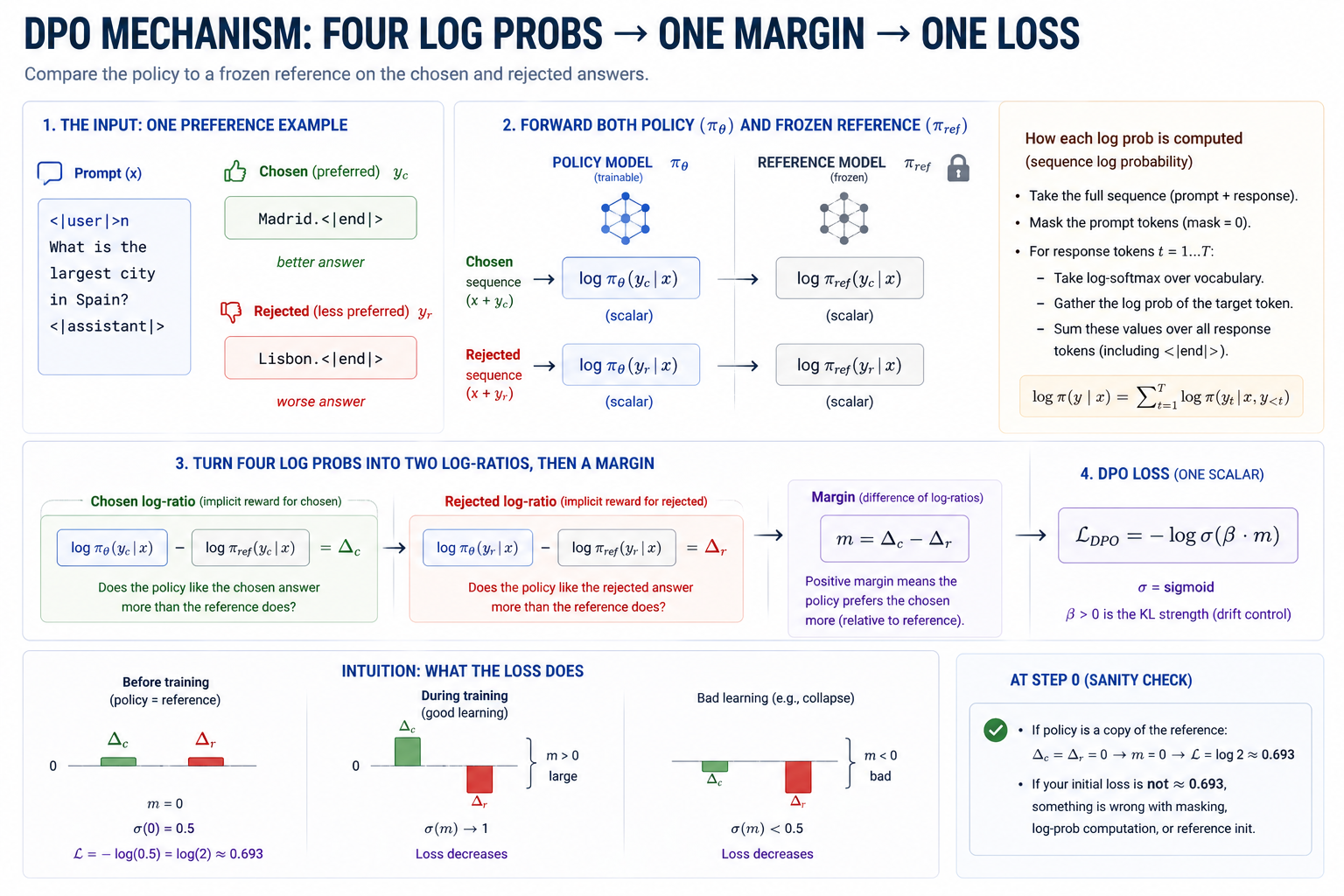 preference triplet → four log-probs → two log-ratios → one margin → one scalar loss.
For a single preference example:
       loss_c = ( log π(y_c | x)  −  log π_ref(y_c | x) )     ← chosen
       loss_r = ( log π(y_r | x)  −  log π_ref(y_r | x) )     ← rejected

       m̂      =  loss_c - loss_r

       L_DPO  =  − log σ( β · m̂ )
m̂ is the policy-vs-reference improvement. β scales that log-ratio margin into an implicit-reward margin. DPO loss is the negative log-likelihood of "chosen beat rejected" under a pairwise preference model.
   ┌────────────────────────────────────────────────────────────────────┐
   │                                                                    │
   │              log π(c|x)  −  log π_ref(c|x)        ┌────────────┐   │
   │              ─────────────────────────────  ──►   │  CHOSEN    │   │
   │              policy / ref ratio for chosen        │  IMPLICIT  │   │
   │                                                   │  REWARD    │   │
   │                                                   └────────────┘   │
   │                                                          │         │
   │                                                          ▼         │
   │                                                       (β · ·)      │
   │                                                          │         │
   │                                                          ▼         │
   │   ┌────────────┐                                  ┌────────────┐   │
   │   │  REJECTED  │   ◄────────────────────────────  │  CHOSEN    │   │
   │   │  IMPLICIT  │    log π(r|x)  − log π_ref(r|x)  │  REWARD −  │   │
   │   │  REWARD    │       (with same β · ·)          │  REJECTED  │   │
   │   └────────────┘                                  └────────────┘   │
   │                                                          │         │
   │                                                          ▼         │
   │                                          loss = − log σ(margin)    │
   │                                                                    │
   └────────────────────────────────────────────────────────────────────┘
At initialization: both ratios are zero, the margin is zero, σ(0) = 0.5, and loss = log 2. This is always the canonical DPO sanity value. If you implement DPO and initial loss is anything else, the implementation is wrong.
As training proceeds: the policy pushes log π(y_c|x) up and log π(y_r|x) down. The reward margin (chosen_reward − rejected_reward) is the main number to watch. If training is working it should gradually increase over the run.
β controls how far the policy can drift from the reference. It is the KL-regularization strength, not the optimizer learning rate — AdamW's step size is a separate knob in the same training loop. Small β (e.g. 0.01) lets the policy diverge a long way for small preference signals. That invites risk of mode collapse, repetition, and gibberish. Large β (e.g. 1.0) pins the policy near the reference — safe but sometimes can't move enough to absorb the preference signal. The DPO paper and most follow-ups recommend β ∈ [0.1, 0.5]. At toy scale β = 0.1 is a fine default, though it's always worth sweeping.
The frozen reference¶
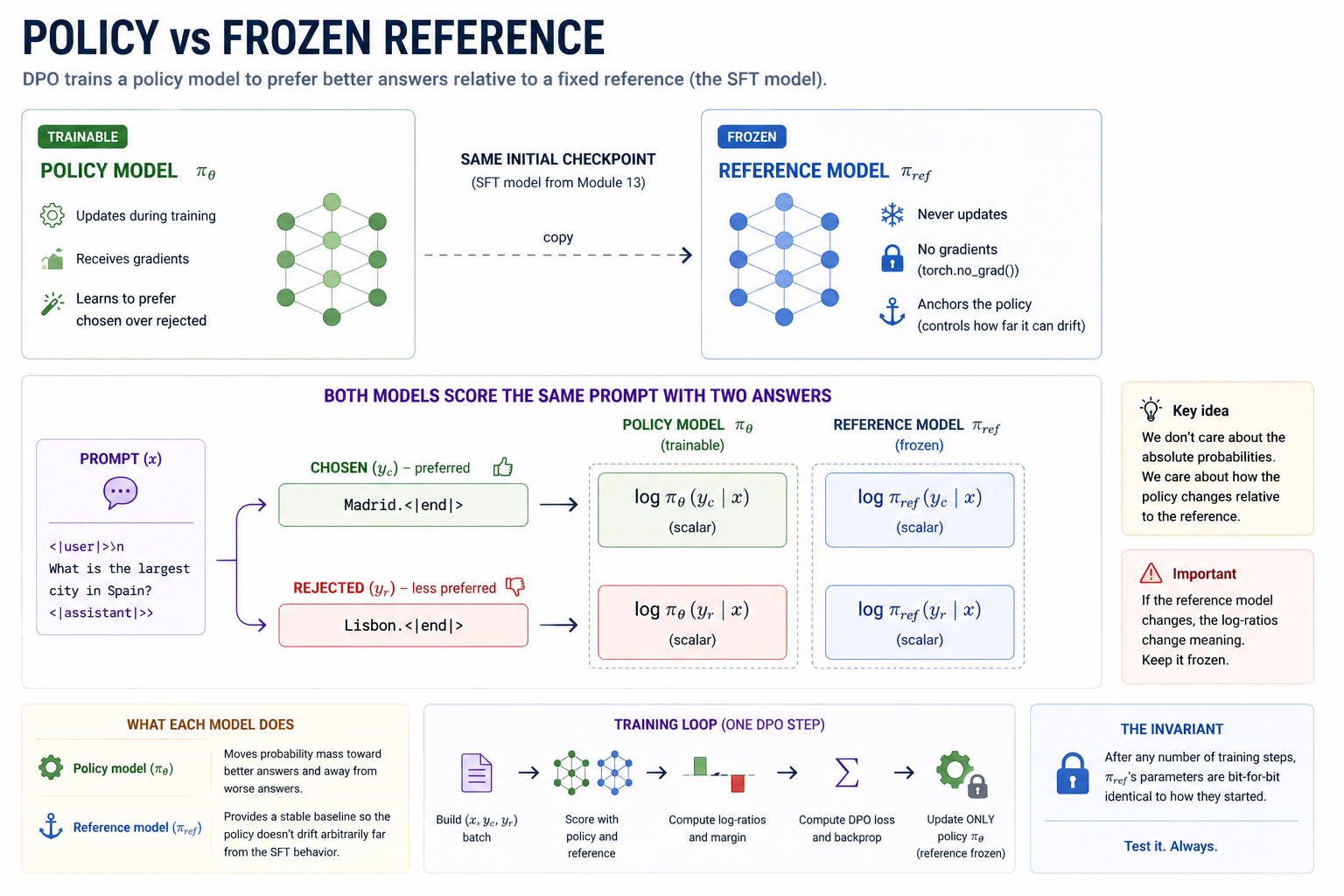 The two-model setup. The SFT model plays both roles — one copy trainable, one copy frozen.
The reference is the anchor for the implicit-reward computation. The whole DPO loss is a function of log-ratios between the policy and the reference. If for some reason both moved together (e.g. an update bug), the log-ratios stay zero and nothing changes.
   ┌─────────────────────────────────────────────────────────────────────┐
   │   POLICY (trainable)                  REFERENCE (frozen)            │
   │   π_θ                                 π_ref                         │
   │     │                                    │                          │
   │     │  forward(prompt + chosen)          │  forward(prompt + chosen)│
   │     ▼                                    ▼                          │
   │   logits_pi_c        ──┐         ┌──   logits_ref_c                 │
   │     │                  │         │       │                          │
   │   log_softmax + gather │         │   log_softmax + gather           │
   │     │                  │         │       │                          │
   │     ▼                  │         │       ▼                          │
   │   logp_pi_c            │         │     logp_ref_c                   │
   │     │                  │         │       │                          │
   │     │       (subtract) │         │       │       (no gradient,      │
   │     │ ◄──────────────────────────│       │        torch.no_grad)    │
   │     │                  │         │       │                          │
   │     ▼                  │         │       │                          │
   │   chosen_logratio = logp_pi_c − logp_ref_c                          │
   │     │                                                               │
   │     ▼                                                               │
   │   (similar for rejected; subtract; multiply by β)                   │
   │     │                                                               │
   │     ▼                                                               │
   │   −log σ(β · margin)                                                │
   │     │                                                               │
   │     ▼                                                               │
   │   backward                                                          │
   │     │                                                               │
   │     ▼                                                               │
   │   ONLY  π_θ.grad  populated;  π_ref  has no grad and no update.     │
   │                                                                     │
   └─────────────────────────────────────────────────────────────────────┘
Preference dataset construction: the costly half of DPO¶
DPO is technically simple but operationally hard because the dataset matters far more than the loss formula. Three construction methods at increasing scale:
-
Hand-authored. You write 50–200
(prompt, chosen, rejected)triples. Slow but high signal — every example is a deliberate choice about what behavior you want the model to prefer. -
Sampled-then-judged. Use the SFT'd model itself to generate two completions per prompt (e.g. with different sampling seeds or temperatures). Have a stronger model judge which is better. The "RLAIF" recipe — reinforcement learning from AI feedback.
-
Static benchmark datasets. Anthropic's HH-RLHF (helpful + harmless), OpenAssistant Conversations, UltraFeedback, etc. Tens of thousands of pairs each. Use only with a stronger base model. Toy-scale models trained on production preference data tend to learn the dataset's biases more than its preferences.
A quality pin for any preference dataset: chosen and rejected should differ in the behavior you care about, not in length, fluency, or surface form. If chosen is systematically longer than rejected, DPO learns "be longer." If chosen uses formal language and rejected uses informal, DPO learns "be formal." Vary only the thing you're trying to teach.
Concepts to internalize¶
- DPO is closed-form supervised loss. The implementation collapses to a single forward+backward per step.
- The policy is the reward model. DPO trains the implicit reward; you can read it off any (x, y) pair after training.
- The reference must stay frozen. If reference updates, the log-ratios do not correspond to learning.
- β controls drift from the reference. Small β: more drift, more risk of collapse. Large β: less drift, less learning.
- The preference dataset format is
(prompt, chosen, rejected)triples. Chosen and rejected share the prompt prefix and diverge over the response. - Sequence-level log-probabilities are sums, not means. A mean would change the objective by length-normalizing.
- At toy scale, 50–200 preference pairs is the right order of magnitude. Not 5; not 5000. Controlling quality is more important than quantity at this scale.
- Length bias is the single most-studied DPO failure. Always check chosen-vs-rejected length distributions before training.
- DPO does not teach new knowledge. Like SFT, it shifts behavior over what the base model already knows. It learns to give more probability to similarly-shaped correct answers, but only when the base model's prior over the relevant tokens already gives them nonzero mass.
What we don't cover¶
- Reinforcement learning from human feedback (RLHF). Largely supplanted by DPO. Still useful when post-training can't be reduced to pairwise comparisons. Worth reading about.
- Online preference collection. Real DPO pipelines iterate: train, sample fresh, grade, append, retrain. This is where most of the engineering effort goes in production models.
- KTO / IPO / SLIC / ORPO and the rest of the DPO-derivative zoo. Each is a small refinement aimed at a specific failure mode (length bias, off-policy drift, the implicit-reward calibration problem). Skim the names; don't implement them.
- LoRA for policy. At production scale, you train a low-rank update on top of the frozen reference. Saves the 2× memory cost. Out of scope here.
- Length normalization. Some DPO variants normalize the log-prob by length. We don't — with similar-length chosen/rejected pairs, length bias is small.
What you'll build¶
Package: g2c/dpo/
class PreferenceExample(NamedTuple):
    prompt_ids:   list[int]                                   # implemented
    chosen_ids:   list[int]                                   # implemented
    rejected_ids: list[int]                                   # implemented


def pad_and_collate_pref(
    examples: list[PreferenceExample],
    *,
    max_seq_len: int,
    pad_id: int,
) -> tuple[
    Tensor, Tensor, Tensor,   # chosen   x, y, mask
    Tensor, Tensor, Tensor,   # rejected x, y, mask
]:                                                            # SCAFFOLDED


def sequence_logprob(
    logits: Tensor,        # (B, T, V)
    targets: Tensor,       # (B, T)
    mask: Tensor,          # (B, T) — 1 where loss applies, 0 elsewhere
) -> Tensor:               # (B,) — per-example log-prob SUM over masked positions
                                                              # SCAFFOLDED


def dpo_loss(
    policy_chosen_logp:   Tensor,   # (B,) WITH gradient
    policy_rejected_logp: Tensor,   # (B,) WITH gradient
    ref_chosen_logp:      Tensor,   # (B,) NO gradient
    ref_rejected_logp:    Tensor,   # (B,) NO gradient
    *,
    beta: float,
) -> tuple[Tensor, dict[str, Tensor]]:                        # SCAFFOLDED


class DPOTrainer:
    model: Module
    ref_model: Module
    examples: list[PreferenceExample]
    beta: float

    def lr(self, step: int | None = None) -> float:           # implemented
    def train_step(self) -> dict[str, float]:                 # SCAFFOLDED
    def evaluate(self, eval_examples) -> dict[str, float]:    # implemented
    def train(self, eval_examples=None) -> dict[str, list]:   # implemented
Total scaffolded code: roughly 60 lines across four locations. The math is light.
How to run the tests¶
Tests live in tests/test_dpo.py. Initial state: 10 passed, 33 failed.
source .venv/bin/activate

pytest tests/test_dpo.py                       # all module-14 tests
pytest tests/test_dpo.py -x                    # stop at first failure
pytest tests/test_dpo.py -k pad_and_collate    # collator tests only
pytest tests/test_dpo.py -k sequence_logprob   # log-prob tests only
pytest tests/test_dpo.py -k dpo_loss           # DPO formula tests only
pytest tests/test_dpo.py -k trainer            # trainer tests only
pytest tests/test_dpo.py -v                    # verbose
Exercises¶
To launch the exercise notebook run:
If at any point you want to archive the work in your current notebook and restart fresh:
The notebook contains the preference-data format, trainer setup, plots, and comparison prompts.
- Hand-author preference data. Create chosen/rejected examples around simple behavior preferences.
- Run DPO. Train policy vs reference and compare SFT/DPO outputs.
- Beta sweep. Study how
betachanges reward margins and drift. - Length-bias injection. Deliberately bias chosen examples and observe the result.
- Reference drift check. Verify the reference model stays frozen.
- Implicit-reward calibration. Check whether DPO rewards rank held-out completions sensibly.
- Optional DPO without SFT. Compare preference training from a base checkpoint.
- Optional malformed rejected example. See how one bad format example can distort behavior.
Pitfalls to expect¶
- Reference model accidentally trains. The reference must be a separate frozen copy. Use
torch.no_grad()for reference forwards. - Prompt tokens in the mask. DPO should score completions, not the shared prompt. Keep the mask on chosen/rejected assistant tokens plus
<|end|>. sequence_logprobshape. DPO needs one summed log-prob per example, shape(B,), before averaging the loss.- Length bias. If chosen completions are systematically longer, the model learns "be longer." Audit pairs before training.
betaextremes.beta=0is a no-op; very large or tiny values can hide whether the policy is actually moving.- DPO loss is not SFT loss. Compare reward margin, preference accuracy, and held-out samples instead of reading DPO loss as a direct quality score.
- Reward collapse. Log chosen and rejected rewards, not just the margin. If both go very negative, lower LR or adjust
beta.
M-series notes¶
DPO is more compute-hungry than SFT but still tractable on M-series:
- Memory is the primary limitation here. With course standard BaseLM, expect to use 6-10GB. Potentially workable with 8GB. Comfortable at 16GB.
- Running time. With BaseLM, the training runs from the exercise notebook should finish in well under an hour.
- Smaller models. The notebook defaults to
BaseLM-SFT. Smaller models from Module 10 are too weak to generalize well, but the same DPO loop runs onTinyLLM,StoryLM, orShakespeareLMif you set the model-selection cell toMODEL_SELECTION = "course"or a specific artifact name.
Reading¶
Primary:
- Rafailov, Sharma, Mitchell et al., "Direct Preference Optimization: Your Language Model is Secretly a Reward Model" (2023). The DPO paper. §4 has the full derivation; the appendix has the gradient analysis. Reading the proof that the closed-form solution to the constrained-RL objective gives the DPO loss is the canonical "aha" moment of this module.
- Ouyang, Wu, Jiang et al., "Training language models to follow instructions with human feedback" (InstructGPT, 2022). The RLHF paper that DPO is a closed-form simplification of. Read §3.4–3.6 for the reward modeling and PPO stages — knowing what DPO replaces makes the simplification feel more dramatic.
- Christiano, Leike, Brown et al., "Deep reinforcement learning from human preferences" (2017). The original deep-RL-from-preferences paper. Predates language models entirely (it's about Atari and Mujoco). Read §2 to see the Bradley-Terry preference model in its pre-LLM form.
Secondary:
- Bai, Jones, Ndousse et al., "Training a Helpful and Harmless Assistant with Reinforcement Learning from Human Feedback" (Anthropic HH, 2022). The HH-RLHF paper. Has the most-cited preference dataset (Anthropic HH) and an extensive discussion of length bias, format bias, and helpfulness-vs-harmlessness tradeoffs.
- Casper, Davies, Shi et al., "Open Problems and Fundamental Limitations of Reinforcement Learning from Human Feedback" (2023). A survey-style critique of RLHF. Read §3 for the failure modes that DPO inherits from RLHF (reward hacking, distributional shift, hard prompts).
- Singhal, Goyal, Xu et al., "A Long Way to Go: Investigating Length Correlations in RLHF" (2023). The length-bias paper. Demonstrates that >50% of the helpfulness improvement RLHF achieves on standard benchmarks comes from length increases alone. Sobering.
Optional:
- Azar, Rowland, Piot et al., "A General Theoretical Paradigm to Understand Learning from Human Preferences" (IPO, 2023). A small refinement of the DPO loss that mitigates an over-fitting failure mode. Read §3 for the analysis of where vanilla DPO breaks; the fix itself is two lines of code.
- Ethayarajh, Xu, Muennighoff et al., "Model Alignment as Prospect Theoretic Optimization" (KTO, 2024). Drops the pairwise structure entirely — train on individual
(prompt, response, label∈{good,bad})examples instead of preference pairs. Useful when pairwise preference data is hard to collect. - Schulman, Wolski, Dhariwal et al., "Proximal Policy Optimization Algorithms" (2017). The PPO paper. RLHF's third stage. We don't implement PPO; reading it once gives you the depth chart of "what DPO is replacing."
- Hejna, Knox, Stone et al., "Inverse Preference Learning" (2023). A different angle on the same closed-form derivation: instead of optimizing the policy directly, recover the reward implied by the policy. Mostly of interpretability interest.
Deliverable checklist¶
- All tests in
tests/test_dpo.pypass. - Hand-authored preference dataset of 100+
(prompt, chosen, rejected)triples indata/dpo/preferences.json(or similar). Length distribution audited - DPO model checkpoint saved to disk, separate from the SFT checkpoint. The SFT checkpoint is preserved for re-runs and ablations.
- One paragraph on what DPO did and what it didn't. The two-list framing is the deliverable; both lists should have at least three items.
- You can explain — out loud, without notes — why the initial DPO loss is exactly
log 2, regardless of architecture, data, or β. - You can explain — out loud, without notes — what the implicit reward is, why it equals
β · log[π/π_ref], and why the prompt's own log-probability cancels. - You can explain — out loud, without notes — why the reference model must stay frozen, what happens if it isn't, and how to verify the freeze invariant.
- You can explain — out loud, without notes — the length bias failure mode and how to detect it before training.