Module 03 — A first neural network

Question this module answers: How do numbers approximate functions?

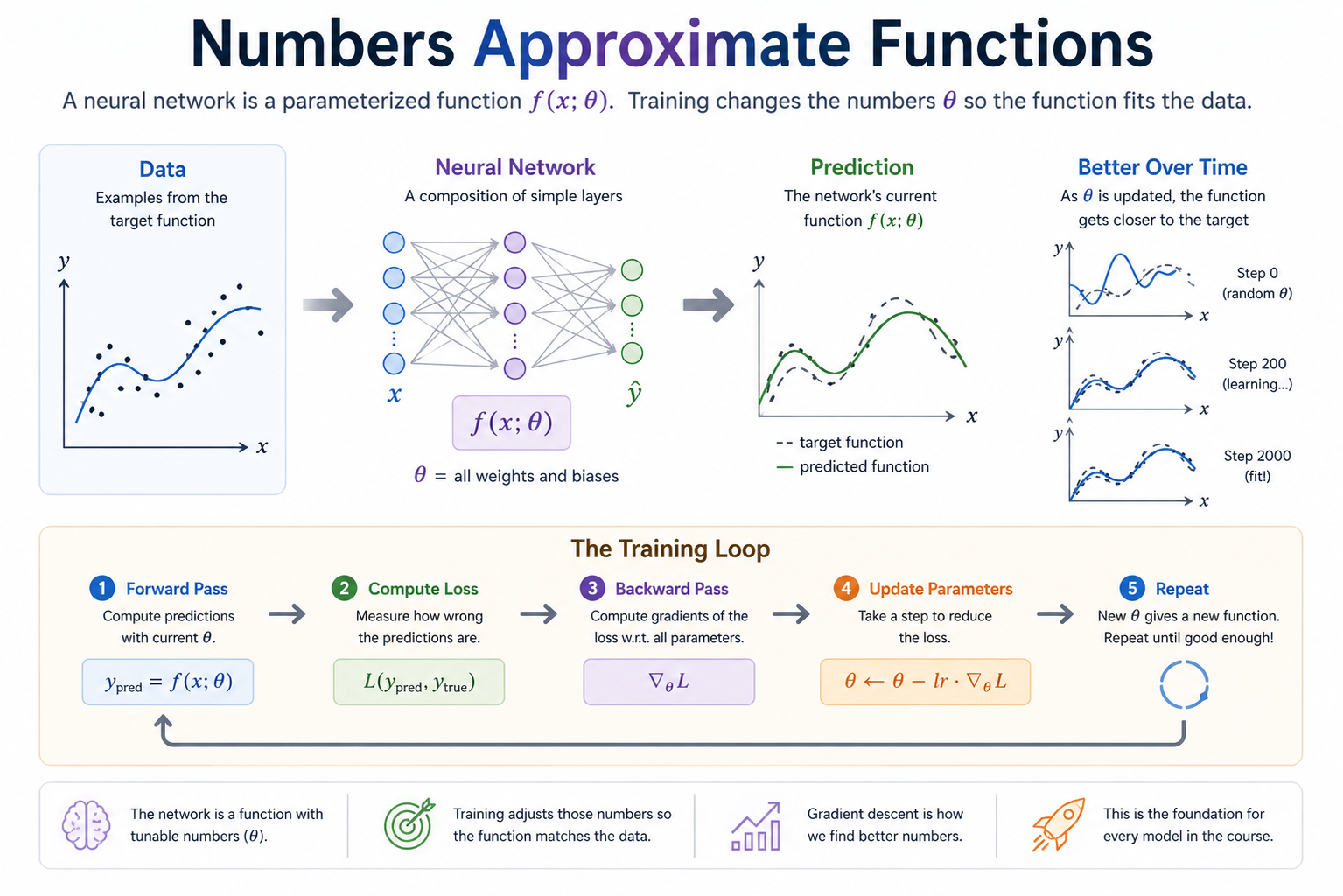
The data, the network, the prediction, and the training loop that closes the gap. Every later module elaborates one of these boxes — attention is a fancier f, RLHF is a fancier L, optimizers are fancier update rules — but the skeleton stays the same.

---

Before you start

• Review 01-autodiff and 02-tensors for the building blocks and 00-prerequisite-review for the basics.
• Review [[PyTorch Primer]] if any of the PyTorch code feels unfamiliar or confusing, especially tensor basics.

---

Where this fits in

Module 01 gave you autograd. Module 02 gave you fast tensor math. Neither, on its own, is a neural network — they're the substrate. Module 03 wires them together into a clean API that looks like a real ML library, and uses that API to train your first model.

The conceptual move is: a neural network is just a parameterized function plus a way to fit it to data. Everything else — depth, layer types, optimizers, schedulers, regularization — is variation on this theme. If you can write a 2-layer MLP that hits >95% on MNIST from scratch, you have the structural understanding required for everything else in the course. The transformer block in Module 09 is the same training loop with fancier layers in the middle.

Concretely, this module has you build:

1. A Module base class plus the building blocks (Linear, ReLU, Tanh, Sigmoid, Sequential).
2. Loss functions (MSELoss, CrossEntropyLoss) — one trivial, one with a real numerical-stability subtlety.
3. An SGD optimizer.

…and use them to fit y = 3x + 2, classify a 2D toy dataset, and finally train an MLP on MNIST.

The big idea

A neural network is a function

f(x; θ) → y

where x is the input, y is the prediction, and θ is a giant bag of parameters (weights and biases). The function is built by composing simple layers — each one a piece of math you can write on a napkin — and the bag of parameters is the union of every layer's parameters.

Training is the loop:

for each batch (x, y_true):
    1. y_pred = f(x; θ)              # forward pass
    2. loss   = L(y_pred, y_true)    # how wrong are we?
    3. ∇θ loss                       # backward pass (autograd does this for us)
    4. θ     ← θ − lr · ∇θ loss      # parameter update (the optimizer's job)

Every layer of every model in this course follows this loop. The variations across the next 17 modules are: what f looks like, what L measures, and what tricks you apply to the update step.

Why nonlinearity is essential

This is the single most important conceptual point in Module 03. Stacking two linear layers without a nonlinearity between them gives you nothing — the composition is still linear:

Linear(in → h) → Linear(h → out)

  y = (x W₁ + b₁) W₂ + b₂
    = x W₁ W₂ + (b₁ W₂ + b₂)
    = x W' + b'                    ← a single linear map

  No matter how many linear layers you stack,
  the composition is one linear layer in disguise.

Insert any nonlinearity (ReLU, tanh, sigmoid) between them and the picture changes completely — ReLU(x W₁ + b₁) W₂ + b₂ is genuinely nonlinear and can approximate arbitrary functions to arbitrary precision (the universal approximation theorem). The whole point of "deep" learning is that nonlinearities make depth pay off.

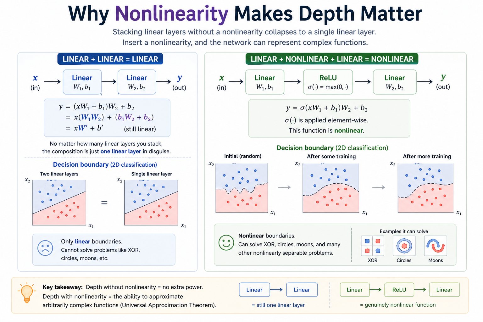Left side: depth without a nonlinearity is the same as width 1 — the algebra collapses, the boundary stays a straight line, and XOR/circles/moons stay unsolvable. Right side: a single ReLU between the layers turns the same architecture into a universal approximator, and the boundary deforms to fit the data. Exercise 5 makes you do exactly this swap and watch accuracy collapse.

Concepts to internalize

• Module as the universal interface. Everything that processes a tensor inherits from it. forward() does the work; parameters() reports learnable tensors. Stacking and composing modules just works.
• Linear layer: y = x W + b. Parameters are W (shape (in, out)) and b (shape (out,)).
• Activations are pointwise and parameter-free. ReLU/Tanh/Sigmoid don't have weights — they're just element-wise functions. They contribute nothing to parameters().
• Loss = scalar. A loss function reduces predictions and targets to a single scalar. Calling .backward() on that scalar populates .grad on every parameter that fed into it.
• Gradient update: param ← param − lr · grad. With weight decay: param ← param − lr · (grad + λ · param).
• Train/val split + overfitting. Always evaluate on data the model didn't train on. Train loss going down while validation loss goes up means the model is memorizing rather than generalizing. Weight decay is the simplest countermeasure.

---

What you'll build

Package: g2c/nn/

modules.py — the building blocks

class Module:
    def __call__(self, *args, **kwargs): ...
    def forward(self, *args, **kwargs): raise NotImplementedError
    def parameters(self) -> Iterable[torch.Tensor]: return []

class Linear(Module):
    def __init__(self, in_features: int, out_features: int): ...
    def forward(self, x: torch.Tensor) -> torch.Tensor: ...

class ReLU(Module):     def forward(self, x): ...
class Tanh(Module):     def forward(self, x): ...
class Sigmoid(Module):  def forward(self, x): ...

class Sequential(Module):
    def __init__(self, *layers: Module): ...
    def forward(self, x: torch.Tensor) -> torch.Tensor: ...

loss.py — loss functions

class MSELoss(Module):           # pre-implemented as a worked example
    def forward(self, predictions, targets): ...

class CrossEntropyLoss(Module):  
    def forward(self, logits, targets): ...

optim.py — optimizers

class SGD:
    def __init__(self, params, lr, weight_decay=0.0): ...
    def zero_grad(self): ...     # pre-implemented
    def step(self): ...          

train.py — small training routines

def train_linear_regression(x, y, steps=500, lr=0.1): ...
def build_2d_classifier(hidden=16) -> Sequential: ...
def accuracy_from_logits(logits, targets) -> float: ...
def train_classifier(model, x, y, steps=1000, lr=0.1, weight_decay=0.0): ...
def build_mnist_mlp(hidden=128, use_relu=True) -> Sequential: ...
def train_one_epoch(model, loader, optimizer, loss_fn) -> float: ...
def evaluate_accuracy(model, loader) -> float: ...

The notebook runs these helpers, but you implement them in the editor so they are covered by tests and survive notebook resets.

A 2-layer MLP, end-to-end

What you'll be able to write once everything is implemented:

Input         Linear         ReLU         Linear         Output
(B, 784)  →  (W₁, b₁)  →  (B, 128)  →  (W₂, b₂)  →  (B, 10)
              W₁: (784, 128)              W₂: (128, 10)
              b₁: (128,)                  b₂: (10,)

  model = Sequential(
      Linear(784, 128),
      ReLU(),
      Linear(128, 10),
  )

Five lines, four parameter tensors, ~100k trainable numbers. Enough to crack MNIST.

How to run the tests

Tests are in tests/test_nn.py. Construction and bookkeeping tests pass from the start; forward passes, losses, optimizer steps, and the training helpers turn green as you implement the TODOs.

source .venv/bin/activate

pytest tests/test_nn.py             # run all module-03 tests
pytest tests/test_nn.py -x          # stop at first failure
pytest tests/test_nn.py -k linear   # only the Linear tests
pytest tests/test_nn.py -v          # verbose

Exercises

To launch the exercise notebook run:

./noteboosh.sh 03

If at any point you want to archive the work in your current notebook and restart fresh:

./noteboosh.sh --fresh 03

The notebook contains runnable experiments and detailed prompts; implementation work lives in g2c/nn/.

1. Linear regression. Fit y = 3x + 2 with Linear, MSELoss, and SGD.
2. Toy classifier. Train a small MLP on a nonlinear 2D classification problem.
3. MNIST MLP. Train the module deliverable and track train/test accuracy.
4. Overfitting and weight decay. Compare a larger model with and without regularization.
5. Remove the nonlinearity. Repeat the 2D circles classifier with and without ReLU() so the boundary collapse is visible.

Pitfalls to expect

• Forgetting torch.no_grad() in SGD.step. The update tensor op gets recorded; the next loss.backward() tries to differentiate through it. you get cryptic RuntimeError or just plain wrong numbers. Always wrap the update.
• Forgetting zero_grad. Gradients accumulate across iterations because PyTorch (like our Module 01 engine) sums .grad rather than overwriting it. Symptom: loss decreases too fast at first, then explodes.
• Naive cross-entropy. Computing (logits.exp() / logits.exp().sum()).log() overflows on real logits. Use the log-sum-exp trick described in loss.py.
• Forgetting nonlinearity. A Sequential of Linear layers with no activation in between is a single linear map dressed up. Won't beat logistic regression on anything nontrivial.
• Using torch.nn.Linear etc. Don't. The whole point of this module is to build them. The same applies to torch.nn.functional.cross_entropy, torch.nn.CrossEntropyLoss, torch.optim.SGD.
• Silent shape bugs. (B, 10) + (10,) broadcasts correctly; (B, 10) + (B,) does not. When the loss is suspiciously flat or NaN, print every tensor's shape first.
• Learning rate too high. Loss explodes to NaN within a few iterations. Cut by 10× and retry.
• Learning rate too low. Loss decreases but glacially. Multiply by 10× and retry.
• Trying to use non-differentiable metrics for training. MSE and cross-entropy are differentiable losses: they tell autograd how to change the parameters. Many accuracy metrics are useful, but non-differentiable and therefore can't be used with autograd. For example average predicted class accuracy.

M-series notes

Everything in this module runs comfortably on a 16GB M-series machine.

• The toy datasets (linear regression, moons, circles) train in seconds on CPU.
• Full MNIST with a small MLP trains in ~1–2 minutes per epoch on CPU.

---

Reading

Primary:

• Karpathy, "The makemore series" lectures 2–4. The most direct mapping to what you're building. Lecture 4 in particular walks through layer composition and a clean training loop.
• 3Blue1Brown, "Neural Networks" series, episodes 1–4. The geometric intuition for what a neural net is doing.

Secondary:

• Goodfellow, Bengio, Courville, Deep Learning, chapters 6 and 7. Textbook treatment of feed-forward networks and regularization.
• PyTorch tutorial: "Build the Neural Network." Useful for seeing how torch.nn.Module works once you've built your own version.

Optional:

• Hornik, Stinchcombe, White, "Multilayer feedforward networks are universal approximators" (1989). The original universal approximation theorem. Skim — the result matters more than the proof.

Deliverable checklist

• All non-skipped tests in tests/test_nn.py pass.
• notebooks/solutions/03-nn.ipynb: 2D dataset, decision boundary plot, working MLP.
• notebooks/solutions/03-nn.ipynb: ≥95% MNIST test accuracy with logged train/val curves.
• Overfitting experiment: train + val curves diverging, then re-converging once weight decay is added.
• You can explain — out loud, without notes — why depth without nonlinearity is still one linear boundary.