Beyond — Manifold-constrained hyper-connections¶

Question this module answers: What if the path around a Transformer block became learnable—and how do you keep that path stable through depth?

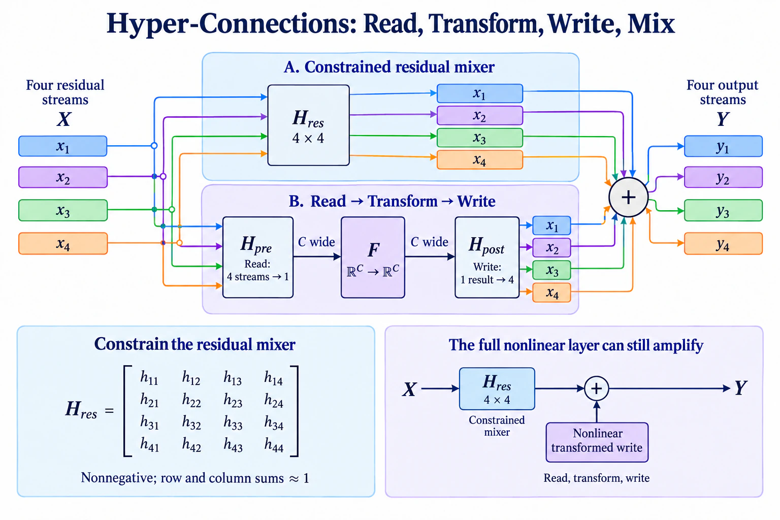
Four residual streams split into a constrained mixing path and a read-transform-write path, then add into four output streams; the mixer constraint does not bound the full nonlinear layer.

Module 09 treated the residual connection as fixed plumbing: normalize one stream, transform it, and add the result back. Hyper-connections turn that plumbing into architecture. They carry several residual streams, learn which mixture a layer reads, how its output is written back, and how the streams exchange information. That extra freedom also creates a new failure mode: unconstrained mixing matrices multiply through depth and can amplify or erase the supposedly safe residual path. This module builds the smallest honest version of manifold-constrained hyper-connections (mHC): multi-stream residual routing, differentiable Sinkhorn projection, and a depth probe that makes the stability constraint visible on a laptop.

This is a Beyond module. Beyond modules sit outside the numbered course: nothing in Modules 00–20 depends on them, and they are not part of finishing the course. Come here in any order, whenever a model card or paper names the idea and you want the load-bearing version — built, trained, and broken on your own machine.

Before you start¶

Review
- 03-nn for tensor modules, parameter initialization, and signal scale
- 09-transformer-block for pre-norm blocks and the ordinary residual connection
Finish
- g2c/nn (03)
- g2c/transformer (09)
- g2c/training (03b) for the optional language-model comparison
Run
- G2C_APPLY_SOLUTIONS=01-10 ./notebook.sh mhc instead of the plain launch if you're entering without your own implementations through the Transformer

Where this fits in¶

Module 09's pre-norm Transformer block has two ordinary residual updates:

x ────────────────────────────────┐
└─ norm → attention ──────────────┴─► x + attention(norm(x))
                                    │
                                    └─ norm → FFN ──► x + attention(...) + FFN(...)

The identity branch is deliberately boring. Even if the learned sublayer starts badly, information and gradients have a direct route around it. Unrolling x_(l+1) = x_l + F_l(x_l) makes that route explicit:

x_L = x_l + Σ F_i(x_i)
      ───
      unchanged path from shallow layer l to deep layer L

Modern models have spent years redesigning the functions inside a block—attention, experts, gates—while leaving this between-block topology almost untouched. Hyper-connections ask whether the residual highway itself can carry more representational capacity. Instead of one C-wide vector, keep n streams of width C; let each layer read a mixture of them, and let its output be written back across them.

That idea now has evidence beyond one paper lineage. DeepSeek V4 and GLM-5.3-Flash both publish mHC residual streams, while separate work has begun testing the mechanism outside language-model pretraining. The recurrence is why mHC earns a Beyond module rather than another paragraph in Module 09. The course version does not reproduce a frontier model: it builds the routing contract and measures the stability property those systems rely on.

The big idea¶

One residual stream becomes several¶

Write the ordinary residual state at layer l as x_l ∈ R^C. A hyper-connection expands it to X_l ∈ R^(n×C): n residual streams, each still C wide. Three small mappings control the topology around an otherwise ordinary layer function F_l:

                         H_pre: read n streams into one
                                      │
                                      ▼
X_l  ── H_res: mix n streams ─────────┼─────────────┐
                                      F_l            │
                                       │             │
                         H_post: write one result    │
                                  into n streams     │
                                       └─────────────┴─► X_(l+1)

In equations:

u_l       = H_pre X_l                              # (C,)
y_l       = F_l(u_l)                               # (C,)
X_(l+1)   = H_res X_l + H_postᵀ y_l                # (n, C)

H_pre     ∈ R^(1×n)     layer read weights
H_post    ∈ R^(1×n)     layer write weights
H_res     ∈ R^(n×n)     residual stream mixer

F_l has the same input and output width as before. The extra topology lives outside it. With n=4, four streams can preserve and recombine different trajectories while each attention or FFN sublayer still processes only one C-wide input.

The mappings can be static learned parameters or dynamic functions of the current token. Production mHC uses both: a static bias plus a small input-dependent projection from the flattened, normalized nC-wide state. This module implements that dynamic form, but initializes the dynamic gates at zero so the model begins from an easy-to-read static residual path.

Why unconstrained routing breaks the residual promise¶

Ignore the writes from F for a moment. After several hyper-connected layers, the old residual state travels through a product of mixers:

X_L = H_res_(L-1) ··· H_res_l X_l + transformed writes
      ───────────────────────────
      composite residual path

An ordinary residual connection has identity on that path. An unconstrained hyper-connection has a product of learned matrices. A singular value slightly above one compounds upward with depth; one slightly below one compounds toward zero. Worse, the largest forward gain and largest backward gain need not occur along the same stream direction.

For a deliberately simple example, repeat one mixer 48 times:

largest gain of H        1.10
largest gain of H^48     1.10^48 ≈ 97

smallest gain of H       0.90
smallest gain of H^48    0.90^48 ≈ 0.006

Real layers use different, input-dependent matrices, so their product is not this scalar arithmetic. The lesson survives: making the bypass learnable removes the fixed identity guarantee. The mHC paper reports precisely this failure at large scale—unstable unconstrained HC runs accompanied by extreme composite routing gains. That is a reported production observation, not something the course's tiny run promises to reproduce.

The constraint: mix without expanding¶

mHC projects each residual mixer into the set of doubly stochastic matrices:

M_ij ≥ 0                 every entry is non-negative
M 1  = 1                 every row sums to one
1ᵀ M = 1ᵀ               every column sums to one

This set is called the Birkhoff polytope. The paper's name says “manifold-constrained”; the particular set used here is more precisely a convex polytope whose corners are permutation matrices.

The constraint buys three concrete properties:

Each output stream is a convex mixture of input streams. A row cannot create an arbitrarily scaled combination.
The mean across streams is preserved. 1ᵀM = 1ᵀ, so averaging after the mix gives the same result as averaging before it.
The guarantee composes. The product of doubly stochastic matrices is doubly stochastic. A deep residual path remains non-negative with row and column sums equal to one.

There is also a useful norm statement. By the Birkhoff–von Neumann theorem, a doubly stochastic matrix is a convex combination of permutation matrices. Every permutation has spectral norm one, so ||M||₂ ≤ 1: the mixer is non-expansive in the stream dimension.

Be exact about what this does not say. A doubly stochastic mixer does not preserve every vector's Euclidean norm; averaging can contract differences between streams. Nor does it force M = I. It preserves the all-ones direction and bounds amplification while still permitting exchange among streams. That conservation path—not a literal unchanged copy of each stream—is the identity-like property mHC restores.

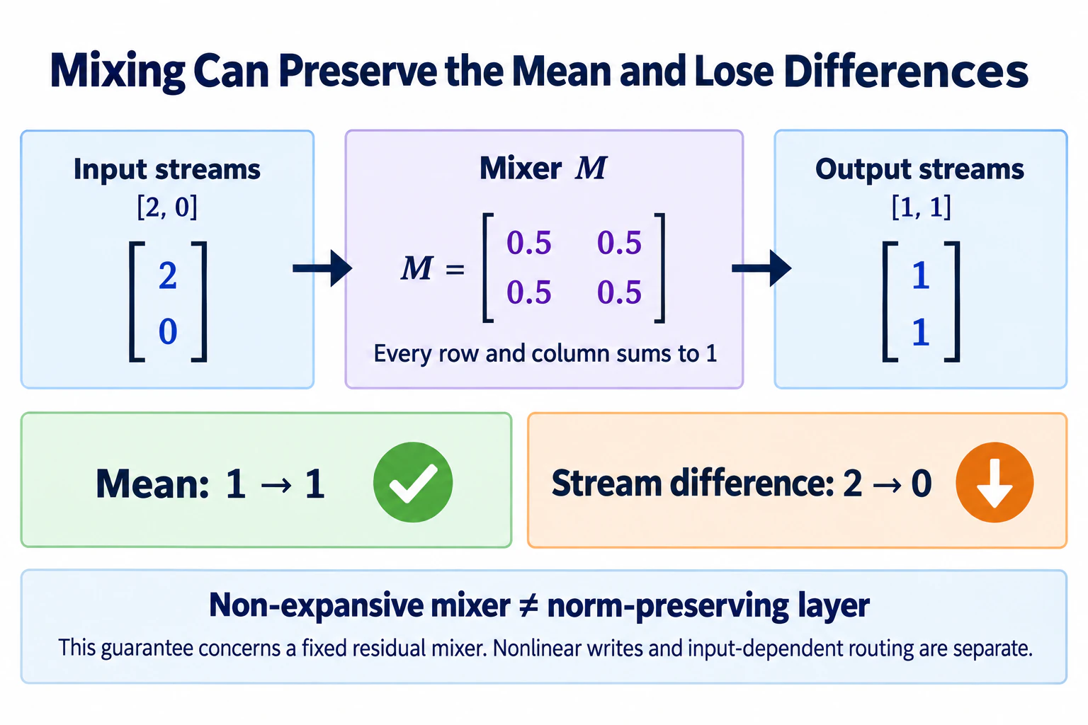A two-by-two averaging matrix maps streams with values two and zero to one and one, preserving their mean while erasing their difference. Doubly stochastic does not mean norm-preserving: this exact mixer preserves the mean but contracts stream differences. The constraint applies to residual mixing, not to the gain of the complete nonlinear layer.

Sinkhorn projection makes the constraint differentiable¶

The model begins with arbitrary routing logits A ∈ R^(n×n). Exponentiation makes them positive, then Sinkhorn–Knopp alternates column and row normalization:

M⁰ = exp(A)

repeat:
    M ← M / column_sums(M)
    M ← M / row_sums(M)

As the iterations continue, both margins approach one. Every operation is differentiable, so a loss can train the routing logits through the projection. The paper uses 20 iterations for its four-stream models. The course implementation also defaults to 20, while the notebook varies the count so you can see that the final-normalized margin is exactest and the other margin still carries approximation error.

Numerical stability matters even for a 4 × 4 matrix. Compute exp(A - max(A)), not raw exp(A), and clamp normalization denominators away from zero. This subtracts one constant from all logits in a matrix and therefore does not change the Sinkhorn result.

arbitrary logits A
        │ exp after max subtraction
        ▼
positive matrix
        │ alternate column / row normalization
        ▼
approximately doubly stochastic M
        │ products stay approximately constrained
        ▼
bounded deep residual mixing

The distinction between exact mathematics and finite implementation is part of the exercise. Exact doubly stochastic matrices are closed under multiplication. Twenty-step projections have small margin error, and multiplication can accumulate it. The right experiment measures that error rather than declaring the numerical matrix exact.

Read, transform, write, mix¶

The full dynamic layer derives all three routing maps from the current multi-stream state. For each batch and token position, flatten X_l from (n, C) to (nC), apply RMS normalization, and make three small projections:

a_pre  = α_pre  · P_pre(norm(vec(X))) + b_pre        # (n,)
a_post = α_post · P_post(norm(vec(X))) + b_post      # (n,)
A_res  = α_res  · P_res(norm(vec(X))) + B_res        # (n, n)

H_pre  = sigmoid(a_pre)                              # non-negative read
H_post = 2 sigmoid(a_post)                           # non-negative write
H_res  = sinkhorn(A_res)                             # constrained mixer

The scalar α gates start at zero. Initially, routing comes entirely from the biases; learning can gradually make it token-dependent. Initialize the read bias so each stream receives weight 1/n, the write bias at zero so 2 sigmoid(0) = 1, and the residual logits close to identity. If all n initial streams are copies of x, the layer begins approximately as n copies of the familiar update x + F(x).

That equivalence is the module's anchor, but it has a limit: after training, the streams need not remain copies, and a learned mHC layer is not merely a standard residual block with extra bookkeeping. Its point is to give depth a learnable routing topology.

Capacity, compute, and the memory wall¶

Because n is small, computing the n × n mixer is cheap beside a Transformer sublayer. That can make “negligible FLOPs” sound like “free.” It is not. The residual activation is nC wide; it must be read, written, saved for backward, and communicated between pipeline stages in a distributed run. The mHC paper reports only 6.7% training-time overhead for its optimized n=4 implementation, but reaches that number with fused kernels, selective recomputation, mixed precision, and communication overlap.

The readable PyTorch implementation in this module has none of those production kernels. Its purpose is to expose the topology, projection, and gradients. On an M-series laptop, expect the mHC toy model to use more activation memory and run slower than the single-stream baseline. That is not a contradiction of the paper's systems result; it is the difference between an algorithm and an optimized deployment.

Concepts to internalize¶

The residual path is architecture. Attention and FFNs are not the only learnable topology in a Transformer; read, write, and between-stream routing can be learned too.
Wider residual state need not widen the expensive sublayer. n streams of width C are read down to one C-wide input for F, then its result is written back across the streams.
Freedom compounds through depth. An unconstrained mixer may look harmless layer by layer while its matrix product explodes or vanishes.
Doubly stochastic means non-negative with both margins equal to one. Rows make outputs convex mixtures; columns preserve the aggregate across streams.
The guarantee is conservation plus non-expansion, not universal norm preservation. Differences between streams may contract, but the mixer cannot amplify the stream-space 2-norm.
Closure is the depth argument. Products of exact doubly stochastic matrices remain doubly stochastic, so the constraint survives composition.
Sinkhorn turns arbitrary logits into trainable constrained routing. Alternating normalizations are differentiable; a finite iteration count leaves measurable approximation error.
Static and dynamic routing are different claims. The production form conditions mappings on the current token. A static matrix teaches the geometry but is not the whole mechanism.
FLOPs are not the whole bill. Widened residual streams increase activation traffic and saved state even when the small routing matrices add little arithmetic.
Model-card literacy: mHC, HC multiplier, residual expansion, Sinkhorn iterations, and doubly stochastic routing describe macro-architecture around the blocks—not an attention variant or optimizer.

What we don't cover¶

Fused mHC kernels. The paper's latency result depends on fused read/write/mix operations. The course uses ordinary PyTorch tensor operations so every mapping remains inspectable.
Distributed activation recomputation and pipeline overlap. These solve memory and communication costs at cluster scale and do not produce a useful single-laptop build.
Alternative constraint sets. Orthogonal, contractive, sparse, or other manifold-inspired residual maps are an open design space. This module isolates the Birkhoff-polytope construction used by mHC.
A theorem that mHC improves language-model quality. The paper reports gains at 3B–27B and larger internal scale. A tiny model can verify invariants and compare optimization behavior, not establish the scaling result.
mHC as parameter-efficient fine-tuning. Later work wraps frozen backbones with residual routing, which asks a different question from changing the pretraining architecture.
Production release reconstruction. DeepSeek V4 and GLM-5.3-Flash combine mHC with MoE, specialized attention, training recipes, and serving systems. This module makes no checkpoint or capability claim about either model.

What you'll build¶

Planned package: g2c/mhc/

def sinkhorn(logits, steps=20, eps=1e-8): ...       # SCAFFOLDED
    # (..., n, n) logits → approximately doubly stochastic matrices

def compose_mixers(mixers): ...                     # implemented
    # multiply a depth sequence of (..., n, n) residual maps

class MHCResidual(Module):                           # boilerplate implemented
    streams: int                                     # n, default 4
    width: int                                       # C
    sinkhorn_steps: int

    def routing(self, x): ...                        # SCAFFOLDED
        # x: (B, T, n, C)
        # return H_pre (B,T,n), H_post (B,T,n),
        #        H_res (B,T,n,n)

    def forward(self, x, layer_fn): ...              # SCAFFOLDED
        # u = H_pre @ x
        # y = layer_fn(u)
        # return H_res @ x + H_post.T @ y

class UnconstrainedHCResidual(MHCResidual): ...       # implemented control
class MHCTransformerBlock(Module): ...                # implemented wrapper
class MHCTransformerLM(Module): ...                   # implemented tiny LM

The pedagogical surface is three functions: project routing logits, construct the dynamic maps, and apply read–transform–write–mix with correct shapes. Constructors, initialization, parameter enumeration, the unconstrained experimental control, and Transformer wrappers are provided. The implementation should remain direct einsum/broadcasting code; optimizing the kernel would hide the object the module exists to teach.

How to run the tests¶

Planned tests: tests/test_mhc.py. Initial target: construction, initialization, and wrapper plumbing pass; tests covering the three scaffolded functions fail with NotImplementedError.

source .venv/bin/activate

pytest tests/test_mhc.py                    # all module tests
pytest tests/test_mhc.py -x                 # stop at first failure (recommended)
pytest tests/test_mhc.py -k sinkhorn        # projection invariants
pytest tests/test_mhc.py -k equivalence     # ordinary residual anchor
pytest tests/test_mhc.py -k gradient        # differentiability and propagation
pytest tests/test_mhc.py -v                 # verbose

The signature test should be test_composed_mhc_mixers_remain_bounded. It composes many projected mixers, checks approximate row and column margins, and verifies that the product's spectral norm does not exceed one beyond numerical tolerance. Paired with an unconstrained control that does amplify, it pins the reason for the constraint rather than only the mechanics of row normalization.

Exercises¶

The planned working notebook is notebooks/clean/mhc-residual-routing.ipynb. To launch it:

./notebook.sh mhc

If at any point you want to archive the work in your current notebook and restart fresh:

./notebook.sh mhc --fresh

Written exercises should live in the notebook as Question: / Answer: cells; ask a coding agent for hints or grading when you're ready, and partial submissions are fine — blank answers are skipped.

Watch Sinkhorn converge. Project batches of random 4 × 4 logits with 0, 1, 2, 5, and 20 iterations. Plot maximum row- and column-margin error. Explain why the margin normalized last is initially more accurate and why both converge.
Multiply through depth. Generate 96 unconstrained near-identity mixers and 96 projected mixers. Track the composite maximum row sum, maximum column sum, and spectral norm by depth. Find a seed where the unconstrained path visibly amplifies or contracts, and explain why a harmless-looking per-layer error compounds.
Read–write routing under a microscope. Feed a hand-constructed four-stream tensor through one mHC layer with a simple linear layer_fn. Inspect H_pre, H_post, and H_res for two different tokens. Trace one output stream numerically back to the streams it read and the transformed value it received.
Break one half of the constraint. Replace Sinkhorn with row-softmax, then repeat the depth probe. Rows still sum to one, so forward values are convex mixtures; columns are free. Measure what happens to the aggregate signal and backward gradients, and explain why row-stochastic alone is not the same contract.
Compare three tiny networks. Train matched-depth single-stream residual, unconstrained-HC, and mHC models on the same small sequence task. Report loss, gradient norms, activation norms, and wall time. The important result is the diagnostic profile, not which validation loss wins.
Written: the activation bill. For batch B, sequence length T, width C, depth L, dtype size s, and stream multiplier n, compare the raw residual-activation elements for the single-stream and multi-stream models. Then explain why the paper's small FLOP overhead does not imply the same memory or bandwidth overhead.
StoryLM comparison (optional). Wrap a shallow StoryLM transformer with four-stream mHC and compare it with the ordinary Module 09 block at a roughly matched training budget. Treat a tie or regression as valid evidence at tiny scale; do not infer the paper's scaling curve from this run.

Pitfalls to expect¶

Using only row softmax. It creates convex output mixtures but does not preserve total contribution from each input stream. The column-margin and composition tests exist to catch exactly this shortcut.
Normalizing the wrong axes. Sinkhorn alternates over the last two matrix dimensions. Accidentally including batch, token, or feature axes can still produce plausible numbers while coupling unrelated examples.
Exponentiating raw large logits. exp(100) creates infinities before normalization can rescue anything. Subtract the per-matrix maximum first.
Detaching inside Sinkhorn. The margins look perfect, but routing projections receive no gradients. The gradient test must reach the original logits and the dynamic routing parameters.
Writing one transformed vector into the wrong axis. H_post distributes y over streams; it does not scale feature channels. Name dimensions in the einsum or insert singleton axes explicitly.
Claiming exact double stochasticity after finite iterations. The final row normalization makes rows especially accurate; columns converge only approximately. Report tolerances and iteration count.
Calling the constraint norm preserving. The all-ones direction and stream mean are preserved, while other directions can contract. The precise guarantee is non-expansion in stream-space 2-norm.
Comparing parameter-matched models and compute-matched models as though they were the same control. mHC adds routing parameters and nC residual activations. State which resource you matched.
Expecting the tiny training run to reproduce frontier-scale gains. The laptop experiment tests implementation, propagation, and optimization clues. It is not an architecture verdict.

M-series notes¶

The projection is tiny. Twenty iterations over 4 × 4 matrices are easy to inspect; no custom Metal kernel is warranted.
The widened activation is the real local cost. Four streams mean roughly four times the raw residual-state elements before saved intermediates. Start with shallow models and short sequences.
Keep the routing math in float32. Mixed-precision production kernels are outside scope, and float32 makes margin and gradient diagnostics easier to interpret on MPS.
Run matrix norms on CPU if needed. torch.linalg.svdvals support and performance vary on MPS; the diagnostic matrices are only 4 × 4.
The core notebook needs no new dataset. Exercises 1–6 use synthetic tensors and the corpus already installed by ./setup.sh; the StoryLM comparison is optional.

Reading¶

Primary:

Xie et al., “mHC: Manifold-Constrained Hyper-Connections” (2025). The mechanism this module builds: multi-stream read/write/mix routing, projection onto the Birkhoff polytope, the stability argument, large-scale experiments, and the systems work needed to keep four streams practical.
Zhu et al., “Hyper-Connections” (2024). The unconstrained ancestor. Read its routing topology first if you want to separate what comes from multiple streams from what the manifold constraint adds.

Current release routes:

G2C Brief — DeepSeek V4. mHC inside a stack that also changes attention, experts, optimization, post-training, and serving.
G2C Brief — GLM-5.3-Flash. A second released family with four residual streams and 20 Sinkhorn iterations; useful evidence that the mechanism has crossed a model-family boundary.

Optional:

Wang & Qiu, “Accelerating Birkhoff Projection for Manifold-Constrained Hyper-Connections” (2026). Why unrolling Sinkhorn is not the last word for either projection accuracy or backward memory. Read after the module, not before implementing it.
Oldenburg et al., “Manifold-Constrained Hyper-Connections for Parameter-Efficient Finetuning” (2026). Tests residual routing as a PEFT axis and reports mixed standalone results—valuable evidence that the mechanism's role changes outside pretraining.