G2C Brief — MiniMax M3.1 Flash: three changes, read from the config

Question this Brief answers: How do you make a 428B model about three times faster without changing its skeleton?

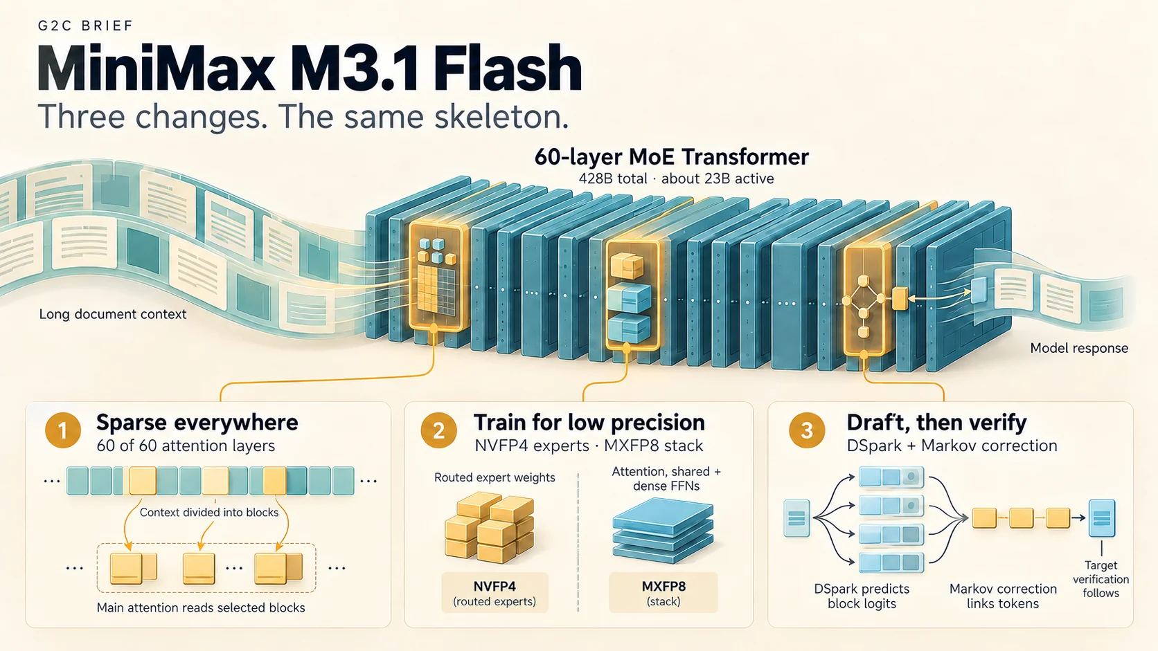
On October 23, 2026, MiniMax published the weights for MiniMax-M3.1-Flash, four days after launching it on its API. It is a mixture-of-experts model with about 428B parameters, 23B of them active per token, a 1M-token context window, and text, image, and video input. MiniMax says it runs "nearly three times faster" than its predecessor, MiniMax-M3, and cuts the cost of agent workloads by about 70%.

There is no technical report for M3.1 Flash, and MiniMax hasn't promised one. What there is turns out to be enough. The model card names exactly three changes from M3:

1. Sparse attention in every layer. M3 kept three layers of ordinary dense attention; M3.1 Flash replaces them.
2. Quantization-aware training. The released weights are 4-bit and 8-bit, and the model was trained to expect that.
3. A new speculative-decoding drafter. DSpark, the drafter introduced with DeepSeek V4.1, replaces M3's own multi-token-prediction modules.

Because both models' weights and configs are public, each claim can be checked by diffing two JSON files and counting tensors, and this Brief does that. The sparse attention mechanism itself has a paper, MiniMax Sparse Attention (MSA), which supplies the explanation the model card leaves out.

For a g2c graduate, each change connects to something you built:

• MSA is attention (Module 07) with a learned selector in front of it, and its speedups follow directly from the prefill-and-decode accounting in Module 16.
• Quantization-aware training is the sequel to Module 16's quantization exercise, where post-training quantization fell off a cliff.
• DSpark's "Markov head" is, almost line for line, the neural bigram model you built in Module 06.

This Brief assumes no background on M3 or on MiniMax.

---

Snapshot

Subject	MiniMax-M3.1-Flash, compared against its predecessor MiniMax-M3
Primary sources	M3.1 Flash model card and config (repo revision 54e4e69); M3 model card and config; MiniMax Sparse Attention (arXiv 2606.13392v2, June 2026); launch post (October 19, 2026)
Weights	Public since October 23, 2026, under the MiniMax Community License: free for non-commercial use; commercial use requires attribution, and written authorization above US$20M in yearly revenue
Technical report	None for M3.1 Flash. The MSA paper covers the attention mechanism, validated on a smaller 109B research model.
Implementation read	TokenSpeed's MiniMax-M3 and DSpark model files, a third-party serving engine listed on the model card. vLLM and SGLang recipes also exist.
Independent evaluation	Artificial Analysis, run against MiniMax's API before the weights were released
Last verified	October 23, 2026

The labels follow the standard Brief meanings, with two notes for this release:

• Derived covers arithmetic from the configs, counts of the published tensors, and statements read from code. When the code is TokenSpeed's rather than MiniMax's, the Brief says so, because a third-party engine can differ from MiniMax's own serving stack.
• Reported claims about M3.1 Flash come from the model card and launch post. Claims about MSA's quality come from the paper's experiments on a 109B model, not on M3.1 Flash itself.

---

The model in one page

Derived, from the config. The text model is a 60-layer Transformer:

Piece	Setting
Hidden size	6,144
Attention	grouped-query: 64 query heads sharing 4 key-value heads (head dimension 128), so each KV head serves a "group" of 16 query heads
Feed-forward	layers 0–2 dense; layers 3–59 mixture-of-experts with 128 routed experts (top 4 per token) plus 1 shared expert, each a SwiGLU MLP of width 3,072
Router	sigmoid scores with a learned bias, the DeepSeek-style balancing scheme
Vocabulary	200,064 tokens
Context	up to 1,048,576 positions
Vision	a 32-layer ViT front end feeding image and video patches into the same stream

Derived. Counting from those settings: the 128 routed experts across 57 layers hold 413.1B parameters. That is 97% of the model. Each token uses 4 of them, so a token touches about 23.5B parameters, excluding the embedding and output matrices. That's the card's "23B activated" figure.

Beyond: MoE builds the routing mechanism at laptop scale. Everything in this section is unchanged from M3. The full diff between the two configs is short:

Config field	M3	M3.1 Flash
sparse_attention_freq (layers using sparse attention)	57 of 60 (layers 0–2 dense)	60 of 60
quantization_config	none (BF16 weights)	NVFP4 routed experts, MXFP8 elsewhere
num_mtp_modules	7	none; a separate dspark/ draft model ships instead
rope_theta	5,000,000	10,000,000
vision_config.image_size	2,016	672

(Derived. The last two rows aren't mentioned on the model card. The RoPE base doubling is the kind of change usually made when retuning long-context behavior; Not disclosed why it changed. The vision setting may only be a default for the processor's tiling. The image grid list is identical in both configs.)

---

Change 1: sparse attention in every layer

What MSA does

Dense attention compares every query with every earlier key. At a 1M-token context that's a million dot products per query, per head, per layer. MSA splits each attention layer into two branches (paper, Section 3):

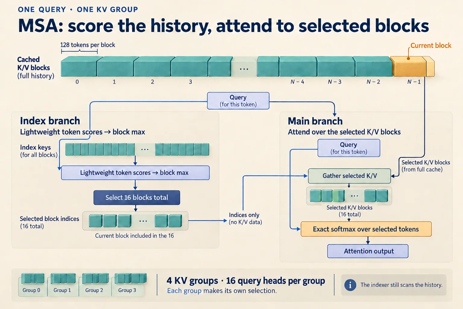Choose where to read before doing the expensive attention. Reported: MSA §3 reserves one of the selected block slots for the local block. Derived: the released config sets 16 blocks of 128 tokens and four KV groups. The illustrated selections are schematic, not measured attention maps.

Three design choices are worth noticing:

• Selection is per KV group, by block. All 16 query heads that share a KV head share one selection. Blocks of 128 consecutive tokens keep the memory reads contiguous. Reported: the paper's ablation found block sizes of 32, 64, and 128 gave nearly identical quality, so the largest, fastest block won.
• The selector learns from the attention it replaces. Top-k is not differentiable, so the language-modeling loss can't train the index branch. Instead, a KL loss pushes the index branch's distribution toward the main branch's actual attention weights, averaged across the group's heads, on the selected tokens. Two stop-gradients confine that loss to the two index projection matrices: the main branch's attention is detached, and so is the index branch's input. The backbone never sees it.
• The selector is warmed up first. For the first stretch of training, both branches run dense attention while the index projections learn. Sparse selection switches on only after the selector has something to go on. Reported: the same recipe converts an already-trained dense model ("near-lossless conversion from pretrained GQA checkpoints").

G2C interpretation. The selector is a student trained by distillation against a teacher that is attention itself. It is the same move as a probe in interpretability, or as Module 15's habit of measuring a cheap proxy against the expensive real thing. The stop-gradient on its input is what keeps it a measurement of the backbone, rather than a second objective bending the backbone to be easier to index.

The config is the paper's final recipe

The paper's appendix ablates several choices, and M3.1 Flash's sparse_attention_config matches each of its conclusions (Derived, config against paper):

Config setting	Paper's finding
sparse_block_size: 128, sparse_topk_blocks: 16	The deployed setting; the top-k kernel is tuned for small k at this block size
sparse_score_type: "max"	Blocks are scored by their maximum token score (max-pooling)
sparse_init_block: 0	No forced "attention sink" block. The model learned to select the first block on its own (Appendix C.2).
sparse_local_block: 1	Only the query's own, partly filled block is forced (Appendix C.2)
sparse_disable_index_value: 1 (every layer)	The index branch's extra output path was removed once warmup made it unnecessary (Appendix C.3)

Reported. The paper's visualizations show what the learned selector picks: every head selects the local neighborhood and the first block (the "sink"), then spends the rest of its budget on a few long-range stripes. Different groups pick different stripes. A fixed sliding window with the same budget had higher perplexity on agent tasks throughout training.

Where the speedup comes from, and where it stops

The paper gives the attention cost of a whole sequence of length N (equation 12). Dividing by N gives an average per token:

   dense GQA:   2 · H_q · d_h · N                  =  16,384 · N
   MSA:         H_kv · d_idx · N  +  4 · H_q · d_h · k · B_k
                └─ index branch ┘    └──── main branch ────┘
             =  512 · N  +  67.1 million

Derived (using M3.1 Flash's settings: H_q = 64, H_kv = 4, d_h = 128, d_idx = 128, k = 16, B_k = 128):

Context N	Dense, per layer	MSA, per layer	Ratio
131,072	2.15 GFLOPs	0.13 GFLOPs	16×
1,048,576	17.2 GFLOPs	0.60 GFLOPs	28.4×

That 28.4× is the paper's headline number, recovered from the formula. Notice the shape of the MSA cost. The main branch is a constant, but the index branch still grows with N: the selector has to look at every block to pick the best 16. Derived: as N grows, the ratio approaches 16,384 / 512 = 32× and never passes it. The index branch is the part of attention that stays quadratic over a whole sequence. It's just 32 times cheaper per key.

Decode tells a different story, because decode is limited by memory reads, not arithmetic (the Module 16 argument). For one decode step at context N, per layer:

   dense GQA reads every cached key and value:   2 · H_kv · d_h · N      = 1,024 · N values
   MSA reads every index key, plus 2,048 tokens   d_idx · N + H_kv · 2,048 · 2 · d_h
   of keys and values for each of the 4 groups   = 128 · N + 2.1 million values

Derived: at a 1M context that's about 1,074 million values against 136 million, a ratio of about 7.9×. Reported: the paper measured a 7.6× decode speedup at 1M on H800 GPUs. The measurement lands right where a pure memory-traffic estimate says it should, which is strong evidence that decode really is a bandwidth problem. The measured prefill speedup is 14.2×, well short of the 28.4× arithmetic ratio. The paper attributes the gap to selection, gathering, and load-balancing overheads that dense attention doesn't have.

What removing three dense layers buys

M3 kept its first three layers dense. That sounds minor: 3 of 60 layers.

Derived. Using the per-token figures above, at a 1M context M3 spends 3 × 17.2 = 51.5 GFLOPs on its three dense layers and 57 × 0.60 = 34.4 GFLOPs on its 57 sparse layers. The three dense layers did 60% of M3's attention arithmetic. M3.1 Flash's 60 sparse layers cost 36.2 GFLOPs in total, 2.4× less than M3's 86. At 128K the dense layers' share was 46%, and removing them cuts attention cost 1.75×.

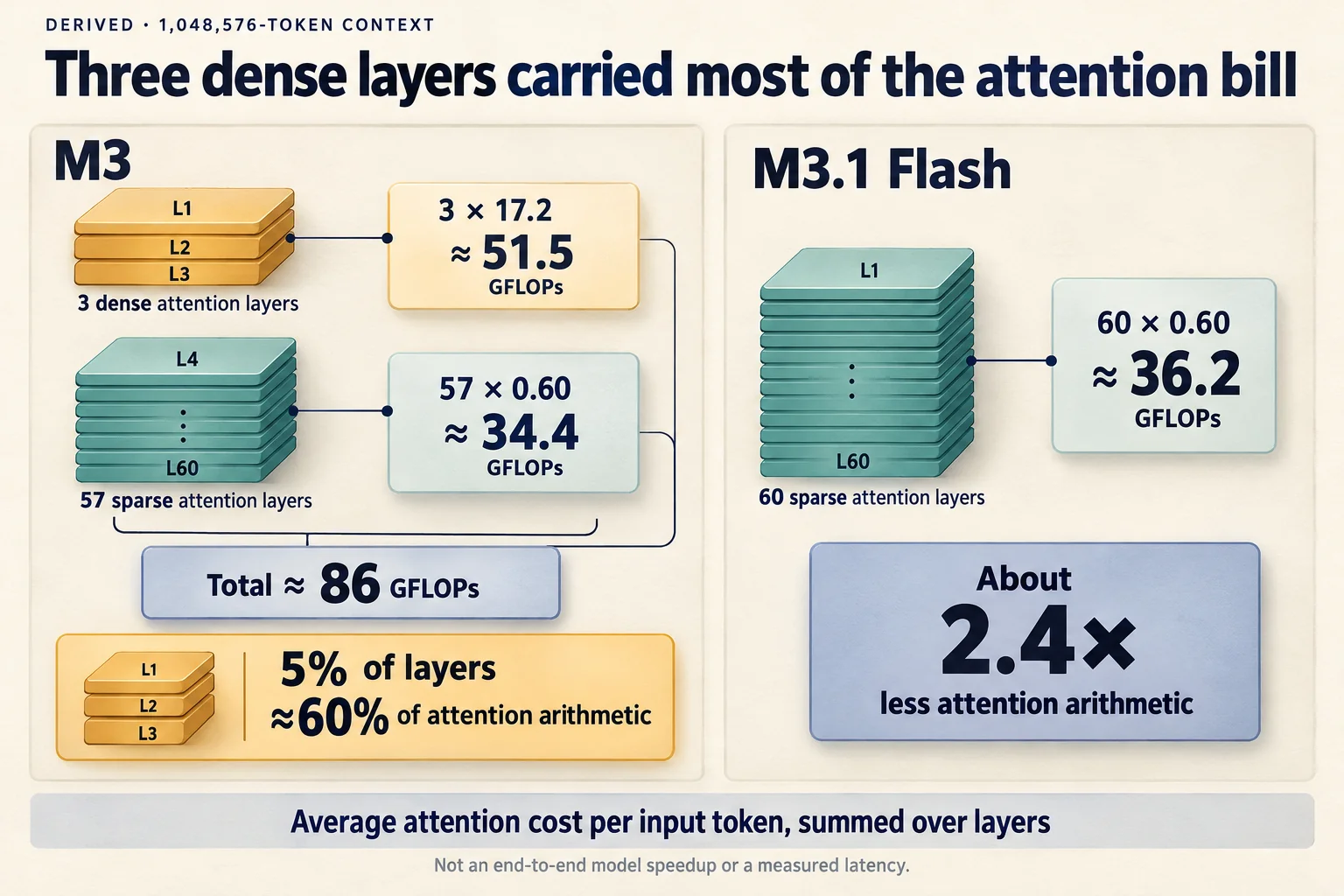Count work, not layers. Derived: the paper's cost equation and released configs put about 60% of M3's attention arithmetic in just three layers at N = 1,048,576. These are average attention FLOPs per input token, summed over layers; the 2.4× ratio is not a measured end-to-end speedup.

For scale, the rest of the network (projections, experts, and so on) costs about 47 GFLOPs per token no matter the context, twice the 23.5B active parameters. At a 1M context, M3's attention alone cost more than the rest of the network. M3.1 Flash's costs less.

Not disclosed: why M3 kept those layers dense, and what removing them cost in quality. The paper's own 109B experiments ran MSA in every layer, so all sparse layers is the configuration the paper actually validated. G2C interpretation: M3's three dense layers look like a production hedge that the team has now judged unnecessary.

What MSA doesn't shrink

MSA saves compute and memory reads. It doesn't save memory. Any block might be selected by some future query, so every key and value must stay in the cache, plus a 128-dimensional index key per token.

Derived. Per token, per layer, the cache holds 2 × 4 × 128 = 1,024 values for keys and values plus 128 for the index key. That's 69,120 values per token across 60 layers. In BF16 that's 138 KB per token, or about 145 GB for one 1M-token sequence. Halve that if the cache is stored in 8 bits. Not disclosed: the precision MiniMax's own serving uses for the cache.

Compare the DeepSeek V4.1-Flash Brief, where the whole architecture was built around a global cache of 890 bytes per token. The efficient-attention map separates the costs that "sparse attention" can mean: the payload cache attended to, the index used to find candidates, and the selection work. G2C interpretation: MSA attacks selection and payload reads. V4.1 attacks payload storage. They are answers to different bills, and a model can need both.

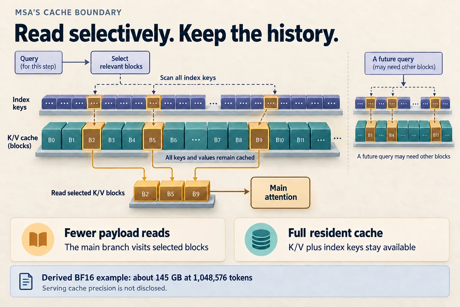Selection changes the reads, not which history must remain available. Derived: the config implies 69,120 cached values per token across 60 layers; at BF16, a full-length sequence occupies about 145 GB. Not disclosed: the cache precision used by MiniMax's service. Weight quantization does not establish cache precision.

---

Change 2: quantization-aware training

What the checkpoint actually contains

Reported. "The routed MoE experts and the attention paths are quantized during training, reducing memory footprint and improving serving efficiency." The config says how:

• Routed experts: NVFP4. 4-bit floating-point values in blocks of 16, each block with its own 8-bit scale factor.
• Everything else in the transformer stack: MXFP8. This covers attention projections, the index branch, the shared experts, and the three dense feed-forward layers. Values are 8-bit floats in blocks of 32, each block with a power-of-two scale.
• Left unquantized: the router gates, the token embeddings, the output head, and the whole vision tower.

Derived. The published tensor counts confirm this split exactly:

Stored as	Elements in the checkpoint	Matches
packed 4-bit (two per byte)	206,561,083,392 bytes = 413,122,166,784 values	128 routed experts × 57 layers × 3 matrices × 6,144 × 3,072, exactly
8-bit float	10,560,208,896	attention + index branch + shared experts + dense FFN layers, exactly
BF16	3,323,222,528	embeddings and output head (2.46B), plus the vision tower and projector

The weight files total 250 GB, against 854 GB for M3's BF16 release (Derived, about 3.4× smaller).

G2C interpretation. The quantization budget follows the parameter count. The routed experts are 97% of the parameters, so they get the most aggressive format. The small, sensitive pieces stay in higher precision. Router gates decide which experts run, and a rounding error there changes which computation happens, not just how precisely.

Why 4-bit experts matter for speed

Recall Module 16's ceiling on decode speed: tokens per second can't exceed memory bandwidth divided by the bytes read per token. For an MoE model, the bytes per token are mostly the active experts.

Derived. Each token reads 4 routed experts in each of 57 layers: 12.9B parameters. In BF16 that's 25.8 GB per token. In packed 4-bit it's 6.5 GB, plus small block scales. Cutting the bytes per token about 4× raises the decode ceiling about 4× on the same hardware, before any change to the architecture.

What "quantization-aware" adds

Module 16's fifth exercise quantizes a finished model after training (post-training quantization, PTQ) and watches quality fall off a cliff as the bit width drops. The weights were learned without any idea they'd be rounded. At low bit widths, the rounding errors are as large as the weights' own fine structure, and they compound through the layers.

Quantization-aware training (QAT) lets the model see the rounding while it learns. The forward pass uses quantized weights. The backward pass needs a gradient through round(), which is zero almost everywhere. The standard fix is the straight-through estimator: pretend rounding is the identity when computing gradients, and keep full-precision "master" weights for the optimizer to update:

w_used = w + (quantize(w) - w).detach()   # forward: quantize(w); backward: gradient flows to w

The optimizer then finds weights that work after rounding, often weights sitting comfortably inside a quantization bucket instead of on an edge.

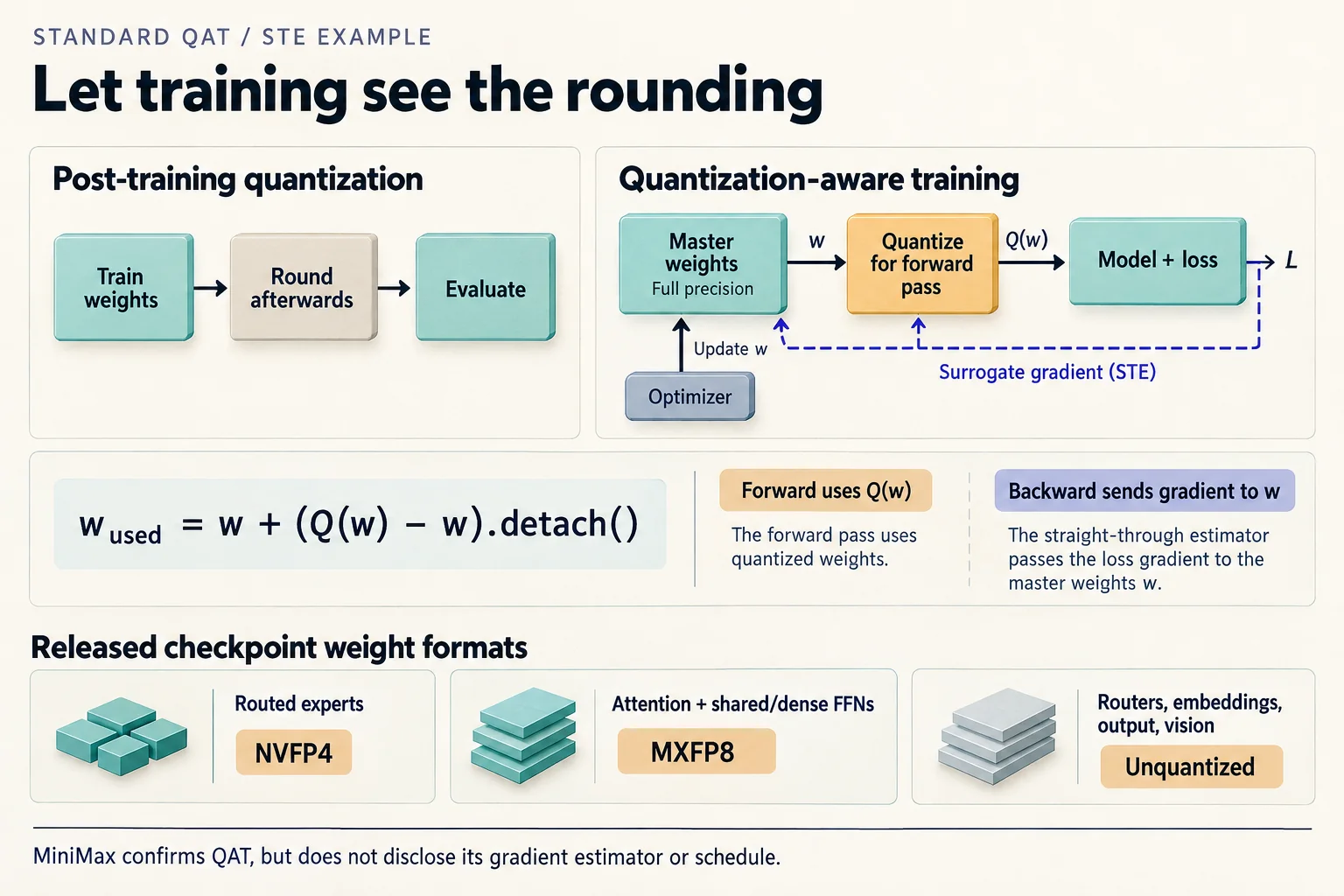Train against the rounding the model will encounter. G2C interpretation: the loop illustrates the standard STE expression above, not MiniMax's disclosed implementation. Derived: the weight-format cards follow the released config. Not disclosed: MiniMax's gradient estimator and QAT schedule.

Not disclosed: MiniMax's recipe. The sources don't say whether quantization ran for all of training or only a final phase, whether it used a straight-through estimator or another method, or how much quality it recovered compared with quantizing M3.1's weights after the fact. The card says only that the experts and attention paths "are quantized during training." For M3, MiniMax published BF16 weights alongside a separate MXFP8 "quantized variant." With M3.1 Flash, the quantized weights are the only weights.

G2C interpretation. That last point has a cost for anyone building on the model. Fine-tuning starts from 4-bit experts, and there's no BF16 master copy to return to. NVFP4 is also a hardware-specific format, with native support on NVIDIA's newest GPUs.

---

Change 3: DSpark replaces multi-token prediction

The drafter

Beyond: speculative decoding builds the core idea: a cheap drafter proposes several tokens, the full model checks them all in one pass, and stochastic verification keeps the target's output distribution exact.

M3 drafted with seven multi-token-prediction modules, which the card calls an "EAGLE-like MTP approach": small modules chained to propose one token after another. M3.1 Flash drops them for DSpark, the drafter DeepSeek introduced with V4.1 (see the V4.1-Flash Brief). The draft model ships in its own dspark/ folder, 2.3 GB.

Derived, from dspark/config.json:

• A small, separate Transformer. It has 5 dense layers at the target's width, using sliding-window attention over the last 4,096 positions.
• It reads the target's mind. Hidden states from five of the target's layers (3, 17, 31, 45, and 59) are concatenated and projected into the draft model as context.
• It drafts a block at once. Positions in a 7-token block are filled with a placeholder "mask" token, and one forward pass predicts all of them in parallel (block_size: 7, mask_token_id).
• A Markov head chains the block back together. Rank 256.
• A confidence head estimates which drafts will survive.

Derived, from TokenSpeed's implementation (third-party). The draft network is non-causal inside the block: every position sees the whole block, including positions after it. That's how one forward pass can fill seven slots.

The Markov head is your bigram model

A single parallel pass has a weakness. Each position predicts its token without knowing what the drafter chose for the position before it. The drafts can be individually plausible and jointly incoherent.

DSpark's fix is small. Derived, from TokenSpeed's code:

markov_w1 = nn.Embedding(vocab_size, 256)               # previous token → 256-dim vector
markov_w2 = nn.Linear(256, vocab_size, bias=False)      # vector → a bias over the vocabulary
bias = markov_w2(markov_w1(previous_token))             # added to that position's logits

The expensive draft network runs once. Then the drafter samples position 1, uses that token to compute a bias for position 2's logits, samples position 2, and so on down the block. The chain is cheap because each step is one embedding lookup and one matrix-vector product.

Compare Module 06's NeuralBigramLM: embed the previous token, apply a linear layer, produce logits over the vocabulary. It's the same model. Here it's used as a correction term instead of a whole language model. Derived: with rank 256, the head has 2 × 200,064 × 256 ≈ 102M parameters. A full bigram table over this vocabulary would need 200,064² ≈ 40 billion entries. The low-rank factorization is the same trade Module 06 made between CountsBigramLM and NeuralBigramLM.

G2C interpretation. The design splits the work by difficulty. Long-range context, which is expensive, is handled once per block by a network that can see the target's hidden states. Local fluency, which is cheap, is handled token by token by a bigram. That's a recognizable pattern: spend heavy compute where the information is, and light compute where the constraint is simple.

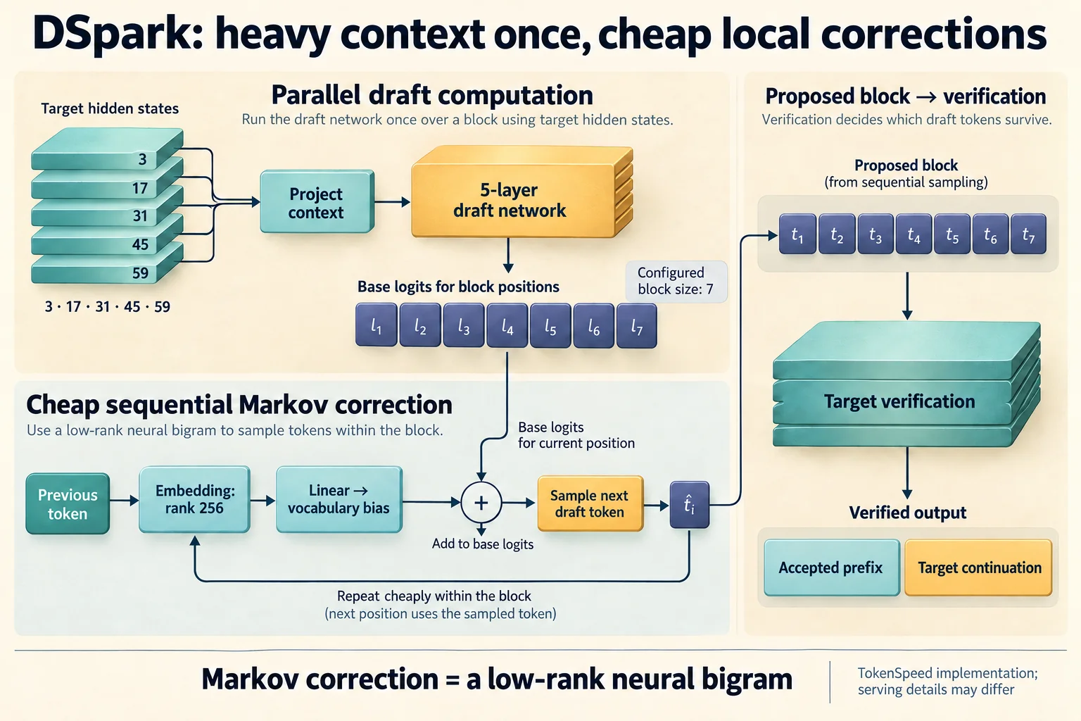One expensive draft pass, followed by a cheap local chain. Derived: the draft config supplies the dimensions and layer taps; TokenSpeed's third-party implementation supplies the Markov correction. The sketch shows the division of work, not an observed acceptance rate or MiniMax's private serving policy.

The confidence head, and who uses it

The draft config sets enable_confidence_head: true, and the checkpoint contains its weights (Derived). That is the head the DeepInfer Brief showed DeepSeek using to budget verification: check only the draft tokens with the best expected return, sized to the current server load.

Derived, from TokenSpeed's code. The open implementation doesn't load the confidence head ("the full block is verified every step"). So the capability ships in the weights, but whether a given serving engine uses it is up to that engine. Not disclosed: whether MiniMax's own service budgets verification, and the acceptance rates DSpark achieves on this model.

G2C note. DSpark is now in production at two independent organizations, DeepSeek and MiniMax, with the drafter's weights and config public for both. Under the Brief rules, that is the recurrence the Beyond-module threshold asks for, and Beyond: speculative decoding already covers the verification side. It's evidence for extending that module to block drafting, not a commitment.

---

Reading the evidence

Reported (model card). Selected results for M3.1 Flash: 73.7% on DeepSWE v1.1, 61.7 on OSWorld 2.0, 76.2 on BankerToolBench, 29.6 on Agents' Last Exam, and 82.2 on CyberGym. The card compares against DeepSeek V4.1 Flash-1017, Kimi K3, GLM-5.3, GPT-5.6 Sol, and Opus 5, with harness and context settings listed per benchmark. Several agentic results use Claude Code as the harness.

Reported (Artificial Analysis, measured against MiniMax's API around launch). The two snapshots available differ slightly:

• Intelligence Index: 42–43, up from 29 for M3. DeepSeek V4.1 Flash-1017 scored 45.
• Cost per index task: about $0.22, down from $0.51 for M3.
• Output tokens to run the index: about 180–189 million. That's well below GLM-5.3 Flash's 324 million.
• Hallucination (via VentureBeat). On AA-Omniscience, the model answered 56% of questions correctly, more than DeepSeek's 43%. But of the questions it didn't get right, 93% got a wrong answer rather than a refusal or a partial answer. It almost never says "I don't know."
• Speed: 87 output tokens per second on MiniMax's API in Artificial Analysis's measurement, against MiniMax's own claim of 170+ (median) and 200+ tokens per second.

G2C interpretation. The cost story has two parts that are easy to blur. The per-token price is low ($0.15 per million input tokens, $0.60 per million output), and the architecture changes plausibly explain why serving is cheaper. But the model also uses fewer tokens per task than its peers, and that is a property of its training, not its attention. Speed numbers depend heavily on load, batching, and whether speculative decoding is tuned for the request mix. Module 16's benchmark section is the right lens: name the phase, the batch, and the context before comparing tokens per second.

The hallucination figure is a calibration finding in Module 15's sense. A model that never abstains can score well on accuracy and still be confidently wrong most of the time when it misses. System prompts and harnesses can sometimes train that out at the application layer. The base behavior is what the number reports.

---

Where informed readers will push back

• The quality evidence for sparse-everywhere is indirect. The MSA paper's experiments are on a 109B model with 6B active parameters, trained for 3T tokens, not on M3.1 Flash. Even there, sparse models trailed dense ones on some long-context subtasks (HELMET-128K retrieval-augmented generation, −2.1; RULER-128K word extraction, −1.35), while gaining on others. Not disclosed: any long-context comparison between M3 and M3.1 Flash, the evaluation that would show what removing the last three dense layers cost.
• A 1M context is still expensive to hold. MSA's savings are in compute and reads. A full-length sequence still needs on the order of 70–145 GB of cache, depending on precision. The card is honest that "usable context length and throughput depend on GPU memory and the serving configuration."
• The QAT recipe is a black box. The release proves what was quantized, down to the tensor. It says nothing about how: when, with what gradient estimator, or at what cost in quality.
• Quantized-only weights narrow who can build on it. There is no BF16 checkpoint. Fine-tuning, distillation, or interpretability research starts from NVFP4 experts and inherits their hardware assumptions.
• Open implementations are partial. TokenSpeed skips the confidence head. Transformers support is "in progress." Reproducing MiniMax's own serving speed depends on implementation details that aren't public.
• Confident wrong answers. The 93% hallucination rate on missed questions is a real deployment concern for any use where an unsupported answer is worse than none.
• The license is not open source. Commercial use requires attribution, and a separate authorization above US$20M in yearly revenue.

---

The laptop boundary, and what you can check yourself

You can't run M3.1 Flash on a course machine. Derived: the weight files alone are 250 GB, four times the largest unified-memory configuration in the course's hardware contract, before any cache. Nothing here asks you to.

Each mechanism, though, has a laptop-sized version. These sketches are optional and ungraded.

Look at your Markov head. Module 06's NeuralBigramLM is the Markov head. Check that its parameter count matches V·D + D·V (plus a bias), then plug in V = 200,064 and D = 256. Then sample a few tokens from it alone. The output is locally fluent and globally aimless, which is exactly the division of labor DSpark relies on: the bigram supplies local fluency, and the draft network supplies everything else.

Compare QAT with Exercise 5's cliff. The straight-through estimator is three lines on top of Exercise 5's fake quantizer. This version uses block scales, as NVFP4 does:

def fake_quant(w, bits, block=16):
    qmax = 2 ** (bits - 1) - 1
    blocks = w.reshape(-1, block)
    scale = blocks.abs().amax(1, keepdim=True).clamp(min=1e-8) / qmax
    return ((blocks / scale).round().clamp(-qmax, qmax) * scale).reshape(w.shape)

def ste(w, bits):
    return w + (fake_quant(w, bits) - w).detach()   # quantized forward, straight-through backward

Use ste(W, bits) in place of W inside a forward pass, fine-tune briefly, then evaluate with fake_quant. In a small trial on a toy two-layer MLP, fine-tuning through ste cut the 2-bit error about 7× compared with quantizing after training, and the 3-bit error about 2×. At 4 bits it made no difference, because block scales already made post-training quantization nearly lossless. Your results on a real language model will differ. The pattern to look for is QAT mattering more as the bits get scarcer.

Measure what a block selector would catch. Take any attention-probability matrix from your own model (Module 07's attention weights, one head, one sequence). For each query, sum the attention mass inside the top-k blocks by max score and divide by the total. This is the paper's "score recall" with a perfect selector:

def topk_block_recall(attn, block=16, k=4):        # attn: (T, T), causal, rows sum to 1
    T = attn.shape[0]
    nblocks = (T + block - 1) // block
    padded = torch.nn.functional.pad(attn, (0, nblocks * block - T))
    per_block = padded.view(T, nblocks, block)
    mass = per_block.sum(-1)                         # attention mass in each block
    score = per_block.amax(-1)                       # MSA scores blocks by their max
    top = score.topk(min(k, nblocks), dim=-1).indices
    return mass.gather(-1, top).sum(-1)              # fraction of each query's attention captured

If a few blocks capture most of the mass, sparse attention would have cost your model little. That's the empirical bet MSA makes at a million tokens.

Redo the arithmetic. Every Derived number in Change 1 comes from three lines of the config and one equation from the paper. Change k, the block size, or the index dimension and watch where the 32× ceiling moves.

---

Coverage map

Mechanism	Coverage	Where
Grouped-query attention, softmax attention	Built in g2c	Module 07, Module 08
Prefill vs decode cost; decode limited by memory bandwidth	Built in g2c	Module 16
Mixture-of-experts routing	Built in g2c	Beyond: MoE
Speculative decoding: draft, verify, accept	Built in g2c	Beyond: speculative decoding
Low-rank bigram model (the Markov head)	Built in g2c	Module 06 NeuralBigramLM
Post-training fake quantization	Built in g2c	Module 16, Exercise 5
Learned block-sparse attention with a distilled selector	Not yet covered	Beyond: Sparse Attention is drafted, not yet buildable; the efficient-attention map explains the payload / index / selection split
Quantization-aware training, straight-through estimator	Conceptual bridge	Module 16's quantization exercise plus Module 01's autodiff
Block formats (NVFP4, MXFP8)	Conceptual bridge	Module 16's quantization section
Block-parallel drafting conditioned on target hidden states	Not yet covered	Beyond: speculative decoding covers drafting one token at a time
Confidence-budgeted verification	Conceptual bridge	DeepInfer Brief; Module 15 calibration

---

A reading route

1. This Brief's "The model in one page" next to the two config.json files. Find the five diff rows yourself.
2. MSA paper, Sections 3 and 5.4. The architecture and the efficiency results. Then Appendix C.2–C.3, the ablations that explain the config.
3. This Brief's arithmetic for the 28.4× and 7.9× figures, redone with your own numbers.
4. dspark/config.json and TokenSpeed's dspark.py (130 lines), next to your Module 06 bigram model.
5. The DeepInfer Brief's Section 4 for what the confidence head is for.
6. Artificial Analysis for the independent numbers, keeping in mind they predate the open weights.

---

After this Brief, you should be able to

• Describe the three changes from M3 to M3.1 Flash and point to the config field that confirms each one.
• Explain how MSA's index branch picks blocks, why it's trained with a KL loss behind stop-gradients, and why it still costs time proportional to the context.
• Derive the 28.4× attention-compute reduction and the roughly 8× decode advantage at a 1M context, and say which Module 16 phase each one belongs to.
• Explain why three dense layers out of sixty were most of M3's attention cost at long context.
• Say what sparse attention does and doesn't shrink, and contrast it with an architecture built to shrink the cache.
• Explain quantization-aware training and the straight-through estimator, and why the routed experts got the most aggressive format.
• Recognize DSpark's Markov head as a low-rank bigram model, and explain how it turns a parallel draft into a coherent one.
• Read a vendor speed claim and an independent measurement side by side, and say why they can both be true.