Beyond — Linear attention and recurrent memory¶
Question this module answers: What changes when token-addressable history becomes a fixed recurrent state?
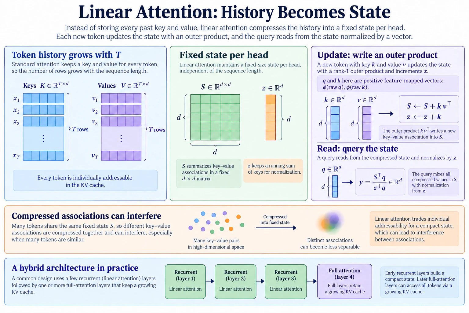
Module 07's attention keeps every past token addressable, and Module 16's KV cache makes that growing history visible. Linear attention takes a more radical bargain: compress the past into fixed recurrent state. This module builds the smallest inspectable version of that bargain, tests its parallel and recurrent forms for equivalence, and measures what a recurrent/full-attention hybrid retains and loses. Use the efficient-attention map for the full taxonomy and Beyond Sparse Attention for the sibling build that retains selected token access.
This is a Beyond module. Beyond modules sit outside the numbered course: nothing in Modules 00–20 depends on them, and they are not part of finishing the course. Come here in any order, whenever a model card or paper names the idea and you want the load-bearing version — built, trained, and broken on your own machine.
Before you start¶
- Review
- 07-attention for the Q/K/V computation this module rearranges
- 16-inference for the KV cache and why its growth is the problem
- Finish
g2c/attention(07 and 08)g2c/transformer(09-transformer-block)g2c/training(03b-training)
- Run
./datasets.sh --tinyif the TinyStories corpus orStoryTokenizerartifact is missingG2C_APPLY_SOLUTIONS=01-16 ./notebook.sh linear-attentioninstead of the plain launch if you're entering without your own implementations through cached inference
Where this fits in¶
In Module 07 we built the all-to-all causal attention contract: every token can consult every previous token. In Module 16 we saw the inference bill that comes with it. A KV cache avoids recomputing old keys and values, but it does not make the history disappear. At history length T, each layer still stores O(T) state and reads and scores O(T) entries for the next token. Over a long generation, that per-token work accumulates.
Long-running agent trajectories and document-scale tasks make that bill increasingly visible. The efficient-attention map compares the distinct responses. Here we follow only the fixed-state branch: a factorizable similarity lets us reassociate attention into a running memory, then selective decay and delta rules show how production descendants make that memory more capable.
The big idea¶
Linear attention starts by replacing softmax attention with a factorizable positive similarity, then changing the order of multiplication. Consider classic attention at one query position t, with the softmax removed for a moment:
   with softmax:      out_t = Σ_i  softmax(q_t·k_i) · v_i      ← must visit every i ≤ t

   without softmax:   out_t = q_t · ( Σ_i  k_i v_iᵀ )
                              ─────   ───────────────
                              (D,)       (D × D)
The entire trick is the reassociation. Σ k_i v_iᵀ doesn't depend on the query. It's just a running sum you can maintain incrementally, with one rank-one update per token:
   S_t = S_{t-1} + φ(k_t) v_tᵀ      # (D, D) state — the "memory"
   z_t = z_{t-1} + φ(k_t)           # (D,)   normalizer
   out_t = (φ(q_t) · S_t) / (φ(q_t) · z_t)
φ is a small positive feature map (we use elu(x) + 1) that provides a factorizable positive similarity in place of softmax's exponentiated dot-product similarity. The result is attention expressed as a recurrent neural network (RNN). The whole past, regardless of sequence length, is compressed into a fixed-size matrix S.
The equations above describe one head and use D for readability. In the multi-head implementation, each head uses d_h = D/H. The complete state is H matrices of shape (d_h, d_h) plus H normalizer vectors: H · d_h² + H · d_h = D²/H + D values, independent of T.
The same computation now has two forms. Implementing both and proving they agree is the module's core deliverable:
   PARALLEL REFERENCE:                 RECURRENT (inference):

   all T tokens at once,               one token at a time,
   explicit T × T decay mask,          carry (S, z) forward
   full teacher forcing, but           O(D²/H) recurrent state work,
   still quadratic in T                O(1) memory in T

          └────────── same numbers, to floating-point tolerance ──────────┘
This mirrors a distinction you have already covered: Module 09's forward trains all positions in parallel, while Module 16's forward_cached generates incrementally. Linear attention makes the incremental attention operation independent of history length. The recurrent state update costs O(D²/H) across the heads; the surrounding dense projections still cost O(D²). The “cache” becomes one fixed matrix per head instead of T growing entries.
There is an important implementation honesty line here. The course's forward uses the full T × T score and decay matrices because that makes the equivalence with step visible. It therefore does not provide linear-time or linear-memory training. Production systems use associative scans, chunking, and fused kernels to expose parallelism without materializing the full matrix. This module demonstrates the fixed-state inference result directly and explains, but does not implement, the production training kernel.
What the compression costs¶
S_t is a compressed summary. Every key-value pair is superimposed into the same fixed matrix, so associations can interfere. Plausible consequences include:
- Exact recall may degrade with distance. Full attention retains an addressable key/value row for every token; the recurrent state superimposes them.
- Copying and induction may weaken. The induction pattern from Module 08 asks for an exact lookup, which is a demanding use of a fixed-capacity state.
- Average next-token loss may hide the difference. If most predictions in a corpus depend on nearby context, a relatively rare retrieval failure contributes little to the average. Exercises 2 and 3 test whether that story actually appears at StoryLM scale.
Fixed decay versus an input-dependent gate¶
The recurrence above is the undecayed γ = 1 case: it never forgets, so early tokens never fade and the magnitudes inside the state can keep growing. This module adds the smallest useful forgetting mechanism to both recurrent accumulators:
With γ_h below 1, every token handled by head h decays that head's old state by the same proportion. This is a fixed learned decay, not a content-dependent gate. It cannot decide that punctuation should be forgotten quickly while a name should persist. Modern gated recurrent layers compute a decay or write strength from the current token. Delta-rule variants also subtract what the state already predicts for a key before writing the corrected value. Those mechanisms are more selective; this module keeps one scalar per head so the recurrence and its parallel reference remain inspectable.
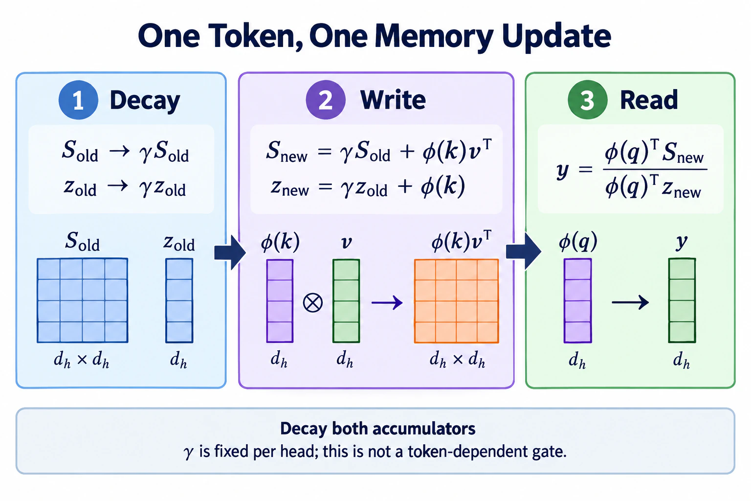 Follow the matrix and normalizer together: decaying only one breaks the parallel/recurrent equivalence you test in the notebook. This fixed per-head decay is the baseline for the more selective writes below.
From fixed decay to KDA's gated delta write¶
The additive update above writes every new association on top of the same finite matrix. If two keys overlap, their values interfere; writing the new value does not first remove the old value that the state associates with that key. A delta-rule layer turns the state into a tiny online learner. In the orientation used by this module, its core can be read schematically as:
prediction_t = k_tᵀ S_(t-1)                         # what memory says for this key
error_t      = v_t - prediction_t                   # what needs correcting
S_t          = G_t S_(t-1) + β_t k_t error_tᵀ      # forget, then corrective write
β_t controls how strongly the new association is written. G_t is a decay gate derived from the current token rather than one fixed γ_h; depending on the architecture it may act per head, per channel, or through a more structured transition. The important distinction is conceptual. Fixed decay says “this head forgets at one learned rate.” A gated delta write says “for this token, decay selected memory directions and change only the part of the association that is currently wrong.”
Kimi Delta Attention (KDA) is a production descendant of this rule. It refines Gated DeltaNet with finer-grained diagonal decay; deployed stacks can surround that recurrence with normalization, short convolution, chunkwise training algorithms, and fused kernels. GLM-5.3-Flash uses KDA for 34 of its 45 text layers. That does not make this module's LinearAttention a toy KDA: the course builds the fixed-state economics and parallel/recurrent equivalence, while KDA's selective transition remains a conceptual bridge.
The hybrid pattern¶
Linear attention compresses history; full attention everywhere pays the full cache. A useful middle point is to stack mostly-linear layers with an occasional full-attention layer:
   layer 12:  linear      ┐
   layer 11:  linear      │  cheap, O(1)-state mixing
   layer 10:  linear      ┘
   layer  9:  FULL        ←  exact token access available; KV cache paid here
   layer  8:  linear      ┐
   ...                    ┘
The full layer makes exactly addressable token identities available to the residual stream; whether one such layer repairs a given task is empirical. The cache bill scales with the number and cache geometry of the full layers. Exercise 5 computes the contrast: at D=4096, one fp16 MHA layer needs about 16.4 GB of KV cache at one million tokens, GQA with eight KV heads needs about 4.1 GB, and one linear layer's (S, z) state is about 1.1 MB. A 3:1 hybrid pays a growing cache in one quarter of its layers, but the size of that cache still depends on whether those layers use MHA, GQA, or another compression scheme.
Concepts to internalize¶
- Linear attention uses a factorizable similarity. Replace softmax with a positive feature kernel, regroup the computation, and each head's past collapses into a running
(d_h, d_h)state. - One computation, two forms. The readable parallel reference and recurrent inference form are equal to floating-point tolerance. The equivalence test is the module's anchor; the reference is not an efficient training kernel.
- The state is a compressed summary. Average loss and targeted recall measure different things; neither experiment's outcome should be assumed in advance.
- A fixed decay is not a selective gate. This module learns one forgetting rate per head. Token-dependent gates can choose what to retain based on content.
- A delta write corrects an association instead of only adding another one. It reads what the state currently predicts for a key and writes the residual error; KDA adds finer-grained, token-dependent decay around that idea.
- Hybrids expose a dial. Full layers retain exact token access and growing caches; recurrent layers use fixed state. The layer pattern chooses where to pay each cost.
- A recurrent layer is one branch of efficient attention. The map keeps its guarantees distinct from exact kernels, compressed token caches, and sparse selection.
What we don't cover¶
- State-space model derivations. Mamba's selective-scan formulation arrives at a similar place from control theory. The convergence is the interesting fact; the HiPPO math is its own course.
- Other efficient-attention families. The efficient-attention map owns FlashAttention, MQA/GQA/MLA, sparse selection, and IndexPool.
- Hardware-aware scan and chunked kernels. Real implementations balance within-chunk parallelism against recurrent state passing. Our readable parallel reference materializes
T × Tscores, so it proves equivalence but does not realize efficient training. - KDA and other gated delta-rule implementations. We trace the corrective write and selective-decay bridge, but keep a fixed per-head decay in the scaffold so the recurrent state and its parallel reference remain inspectable.
- Recurrent-state commit and rollback. A fixed summary has no token rows to truncate after rejected speculative drafts. Beyond Speculative Decoding explains checkpoint-plus-input replay as the serving bridge; neither module builds the production kernel.
- Position embeddings under recurrence. How RoPE-style rotations interact with state-based attention is a genuinely fiddly topic we sidestep by keeping Module 09's learned positions.
What you'll build¶
Package: g2c/linear_attention/
def feature_map(x): ...                  # implemented — elu(x) + 1

class LinearAttention(Module):
    embedding_dim: int
    num_heads: int
    # same Q/K/V/output projections as Module 08
    gamma_logit: torch.Tensor            # (H,) learned parameter
    decay: torch.Tensor                  # property: sigmoid(gamma_logit)

    def parameters(self): ...                                   # implemented
    def forward(self, x): ...                                   # SCAFFOLDED
        # parallel reference: explicit decayed T × T scores, all
        # positions at once; readable, but not an efficient train kernel
    def step(self, x_t, state): ...                             # SCAFFOLDED
        # recurrent/inference form: one token in, (S, z) carried
        # forward, one token out — must match forward() exactly

class HybridBlock(Module):               # Block with attn ∈ {full, linear}   # implemented
class HybridTransformerLM(Module):       # TransformerLM over a layer pattern  # implemented
    # pattern like ["linear", "linear", "linear", "full"] * repeats
Total scaffolded code: roughly 35 lines across two methods. forward and step are two views of one computation; when the equivalence test passes, you've understood the module.
How to run the tests¶
Tests live in tests/test_linear_attention.py. Initial state: 8 passed (the provided feature map, construction, state shapes, accounting, and hybrid stacking), 7 failed.
source .venv/bin/activate

pytest tests/test_linear_attention.py              # all module tests
pytest tests/test_linear_attention.py -x           # stop at first failure (recommended)
pytest tests/test_linear_attention.py -k equiv     # parallel-vs-recurrent equivalence
pytest tests/test_linear_attention.py -k causal    # causality tests
pytest tests/test_linear_attention.py -v           # verbose
The anchor test: test_parallel_matches_recurrent runs the same sequence through forward and through repeated step calls and asserts the outputs agree. Mismatched normalization, state updated in the wrong order, or decay applied in only one form fails this test with a large, readable error. test_forward_matches_undecayed_reference_at_gamma_one separately prevents both forms from agreeing on the same unnormalized computation.
Exercises¶
To launch the exercise notebook run:
If at any point you want to archive the work in your current notebook and restart fresh:
Written exercises live in the notebook as Question: / Answer: cells; ask a coding agent for hints or grading when you're ready, and partial submissions are fine — blank answers are skipped.
- Prove the equivalence, then benchmark decoding. Verify parallel/recurrent equality. Compare one cached full-attention decoding step against one linear recurrent step over growing history lengths, with MPS synchronization and memory arithmetic. Report the observed crossover, including “none in this range.”
- Train the three-way comparison. Train StoryLM-1M full attention, pure linear, and
[linear, linear, linear, full]models on the 100MB TinyStories tier with near-identical parameter counts, batches, and step budgets. Compare validation loss and generated stories. - The recall probe. Train the same three architectural patterns on a synthetic key-value task and measure answer accuracy by retrieval distance. Treat every curve as data: explain what occurred rather than repairing it into the expected narrative.
- Inspect decay. Compare state norms under fixed decay values, then inspect the per-head decays learned by the TinyStories models. Explain what a fixed per-head decay cannot do that an input-dependent gate can.
- Written: four versions of the 1M-token bill. At
T=1M,D=4096,H=32, compare the course's MHA cache, GQA with eight KV heads, an MHA layer retaining a 4096-token sliding window, and linear(S, z)state. Then total the four-layer all-MHA and[L,L,L,F]toy stacks and identify which states still grow withT. - StoryLM-5M rerun (optional). Repeat the TinyStories comparison at the StoryLM-5M architecture. It remains laptop-sized but makes the three-run block substantially longer.
Pitfalls to expect¶
- Dropping the normalizer
z. Outputs drift in scale with sequence length; training limps. Parallel/recurrent equivalence alone cannot catch an omission made in both forms, buttest_forward_matches_undecayed_reference_at_gamma_onepins the normalized result explicitly. - State update order. Whether you update
(S, z)before or after computing the current token's output is the alignment seam: update-first lets a token attend to itself (correct, matching the parallel form); output-first silently shifts everything by one. The equivalence test pins this convention. Causality alone only proves that the future cannot affect the past. - Applying decay in one form but not the other. The parallel form must implement the same geometric decay as
step— via distance-dependent weightsγ^(t-i)— or the equivalence test fails only forγ < 1, which reads as a mystery. - Timing asynchronous MPS work without synchronization. The Python timer stops before Metal finishes and produces fiction. The notebook synchronizes before and after every measured region.
- Comparing training and decoding timings. A full teacher-forced pass and one recurrent token answer different questions. Exercise 1 compares one-token decode paths; the lesson separately explains why this module's training reference remains quadratic.
- Promising a crossover or recall curve. Kernel overhead, context range, optimization, and random seed all matter. “No crossover observed” and “hybrid did not recover the gap” are valid results when supported by the measurement.
- Judging by average loss alone. Even if losses are close, a targeted probe may separate the models; if it does not, that is also evidence about this model and task scale.
M-series notes¶
- Train with the parallel reference only. The recurrent
stepin a Python loop throws away teacher-forcing parallelism. The reference is still quadratic inT; efficient linear-attention training needs a scan/chunk kernel outside this module's scope. - The equivalence check is CPU-comfortable; the full recall probe is a several-minute training block. Its models and sequences are small, but the required path trains three four-layer variants for 600 steps. MPS is recommended for that cell.
- Exercise 2's three StoryLM-1M runs are the compute cost of the required path. StoryLM-5M is an optional rerun. Plug in for either sustained training block.
- MPS and the parallel reference. Its explicit score and decay matrices can be memory-hungrier than standard attention at the same
T. If memory pressure bites, halve the batch before shrinking the model.
Reading¶
Linear and recurrent core:
- Katharopoulos, Vyas, Pappas, Fleuret, "Transformers are RNNs" (2020). The reassociation trick, the feature map, and the parallel/recurrent duality — this module is §3 of this paper, built. Read it first for the implementation branch.
- Schlag, Irie, Schmidhuber, "Linear Transformers Are Secretly Fast Weight Programmers" (2021). Reframes the state as a fast-weight memory and introduces the delta-rule update — the error-correcting write behind the DeltaNet/KDA lineage.
- Gu, Dao, "Mamba: Linear-Time Sequence Modeling with Selective State Spaces" (2023). The state-space route to the same destination. Read for the convergence, skim the derivations.
Further bridges:
- Yang, Kautz, Hatamizadeh, "Gated DeltaNet" (2024). Decay gating plus the delta rule; the cleanest bridge from this module's code to the mechanism used in Qwen3.5's linear-attention layers.
- Kimi Team, "Kimi Linear: An Expressive, Efficient Attention Architecture" (2025). KDA's finer-grained diagonal decay and its chunkwise algorithm. Read the recurrence for the bridge; do not mistake the fused implementation for this module's reference code.
- Sun, Dong, Huang et al., "Retentive Network" (2023). An independent derivation of decay-gated linear attention; useful second angle on why the decay is load-bearing.
Optional:
- 2026 release examples. Kimi K3 reports 69 KDA and 24 Gated-MLA layers, arranged as a 3:1 hybrid plus a final MLA layer. The official Qwen3.5-9B model page reports eight repeats of three Gated DeltaNet layers followed by one gated full-attention layer. GLM-5.3-Flash publishes a
[KDA,KDA,KDA,DSA] × 11 + KDAweave and adds IndexPool on the sparse index. These are production descendants of the fixed-state/full-attention trade, not reproductions of this module's update rule. - Gu, Goel, Ré, "Efficiently Modeling Long Sequences with Structured State Spaces" (S4, 2021). Where the SSM lineage began, if the control-theory route appeals.
Deliverable checklist¶
- All tests in
tests/test_linear_attention.pypass — the parallel/recurrent equivalence especially. - Notebook: honest cached-decoding benchmark (Exercise 1), StoryLM-1M three-way comparison with generated stories (Exercise 2), and empirical recall-vs-distance probe (Exercise 3).
- Written answer for the 1M-token memory bill (Exercise 5).
- You can explain — out loud, without notes — what reassociating
(qKᵀ)Vintoq(KᵀV)buys, and what the softmax's removal costs. - You can explain — out loud, without notes — why hybrid stacks exist, in terms of what the recurrent state cannot do.
- You can explain — out loud, without notes — why this module's recurrent inference state is fixed-size while its readable parallel training reference is still quadratic.
- You can explain — out loud, without notes — how a fixed per-head decay differs from an input-dependent gate.
- You can explain — out loud, without notes — how a delta-rule write corrects the state's current prediction, and why this module does not claim to implement KDA.